Seeking the Tootbird

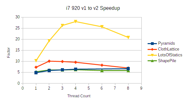
(This post is long! To avoid hiding the release announcement: bepuphysics 2.4 recently released! It's really fast!)

For bepuphysics2's collision detection, I needed a quick way to get a direction of (local) minimum depth for the more difficult convex collision pairs. Minkowski space methods based on support functions are common in collision detection, but the most popular algorithms don't quite cover what I wanted... So after a long journey, I found something (potentially) new. This is the journey to the tootbird.

If you're already familiar with GJK/MPR/EPA and just want to see descriptions of maybe-novel algorithms, you can skip a few sections ahead.

Background

Minkowski space collision detection methods are pretty handy. With nothing more than a function that returns the furthest point on a convex shape along a direction, you can do all sorts of useful things- boolean intersection testing, finding collision normals, separation distance, ray testing, and more.

Thanks to existing good explanations of the basic concepts, I'll skip them here.

The most common algorithms in this space are:

1. Gilbert-Johnson-Keerthi (GJK): Covered by the video above. Many variants exist; specialized boolean, ray, distance, and closest point queries are some of the more frequently seen uses. Often used to find closest points for 'shallow' collision detection with contact manifolds that are incrementally updated from frame to frame. Limited usefulness when shapes intersect; doesn't directly provide a local minimum depth.
2. Expanding Polytope Algorithm (EPA): Sometimes used for finding penetrating depths and collision normals. Conceptually simple: incrementally expand a polytope inside the minkowski difference by sampling the support functions until you reach the surface. It can be numerically tricky to implement and is often much slower than other options. When it is used, it is often as a fallback. For example, using GJK for shallow contact means that only deep intersections need to use EPA.
3. Minkowski Portal Refinement (MPR): From Gary Snethen, a different form of simplex evolution. For more information about how it works, see his website and the source, Pretty quick and relatively simple. As in GJK, variants exist. Boolean and ray queries are common, but it can also provide reasonably good estimates of penetration depth and normal for overlapping shapes. It doesn't guarantee convergence to depth local minima, but it often does well enough for game simulation- especially for simple polytopes that don't have any extreme dimensions.

EPA is pretty rare these days as far as I know (incorrect!). The old bepuphysics1 used GJK for shallow contact with MPR as a deep fallback, optionally re-running MPR in the deep case to (sometimes) get closer to local minimum depth when the first result was likely to be noticeably wrong. It worked reasonably well, and caching the previous frame's state and results kept things pretty cheap.

Motivations in bepuphysics2

I had some specific goals in mind for bepuphysics2 collision detection:

1. One shot manifolds. Bepuphysics1 incrementally updated contact manifolds, with most pairs adding one contact per frame. There are ways to generate full manifolds with GJK/MPR and friends without resorting to feature clipping, but they typically involve some type of sampled approximation. I wanted the same level of quality and consistency that box-box face clipping offered whenever possible. Realistically, for most pairs, this meant manually clipping features against each other.
2. Deeply speculative contact constraints. The algorithm needs to be able to find an axis of (at least locally) minimum penetration depth at any depth or separation. Contact features could then be found from the minimum depth axis.
3. Vectorization. Multiple lanes of pairs are tested at once, scaling up to the machine execution width. This speeds up simple cases enormously, but makes complex state machines or jumping between algorithms like bepuphysics1 did impractical. I needed something that would work across the penetrating and separating cases cleanly.
4. Minimize weird tuning knobs, wonky behaviors, and content requirements. Any method used should be numerically stable and provide local minimum depths such that a user never sees shapes getting pushed out of each other along an obviously suboptimal direction.

Taken together, these goals aren't a good fit for the common Minkowski space approaches. For all collision pairs where it was feasible, I made special cases. Cylinders finally crossed the complexity event horizon, so I began looking for alternatives.

Gradient Methods

In the era of backprop, differentiable systems spew from every academic orifice. I figured I might as well give it a try even if I didn't expect much. It technically worked.

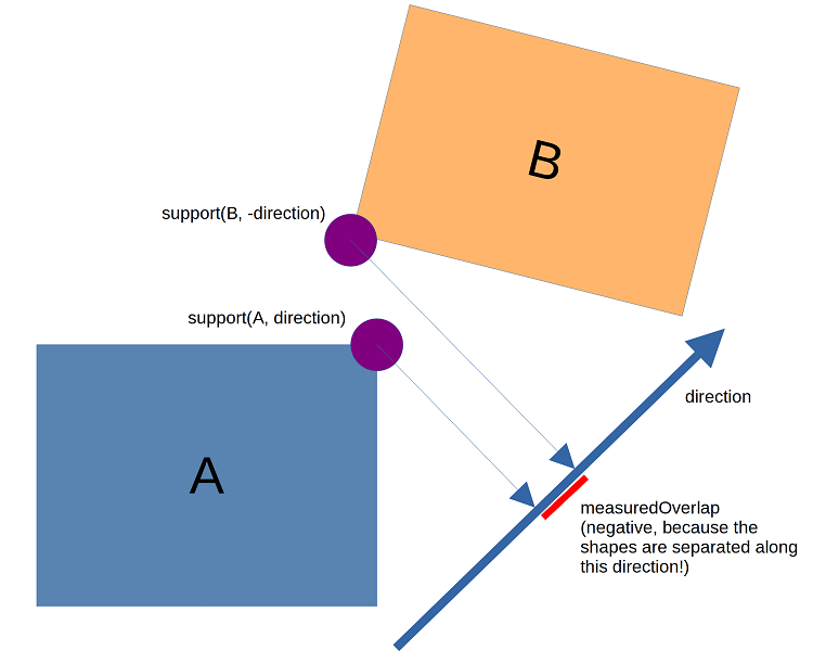
Conceptually, for two convex shapes, there exists a function expressing the depth measured along a given axis: measuredOverlap = dot(direction, support(shapeA, direction) - support(shapeB, -direction)) where support is a functioning returning the extreme point on the given shape in the given direction. The right side of the dot product is the Minkowski difference sample for the direction, but you can also intuitively think of it as just measuring the interval of overlap:

In a gradient based method, we want to repeatedly nudge the direction such that the depth gets lower. For some shapes, mainly those with nice smooth continuous surfaces, you can compute an analytic gradient that is reasonably informative. In those cases, convergence can be quick. But convex hulls and other shapes with surface discontinuities make convergence more difficult. The depth landscape tends to have a lot of valleys that make the search bounce from wall to wall rather than toward the goal, and getting an informative gradient can require numerically constructing it from multiple samples.

Nelder-Mead, an older numerical approach that doesn't require explicit derivatives, ended up being one of the more reliable options I tried.

I did not try any of the newer gradient methods (Adam and beyond); there's room to do better than my early experiments. They would help avoid some of the worst oscillation patterns that naïve gradient descent exhibits in valleys. Unfortunately, even with that, I suspect the iteration counts required for the target precision would become prohibitive. The above video uses 51 support samples to converge. Stopping early tends to yield noticeably bad behavior.

Poking Planes

Desiring alternative direction update rules, I scribbled on paper for several hours.

A newt notices something.

The support function for the Minkowski difference forms a support plane. If you think of the support point as a fulcrum and push the plane toward the Minkowski space origin in the overlapping case (the origin is contained in the Minkowski difference), you make progress towards a local minimum depth.

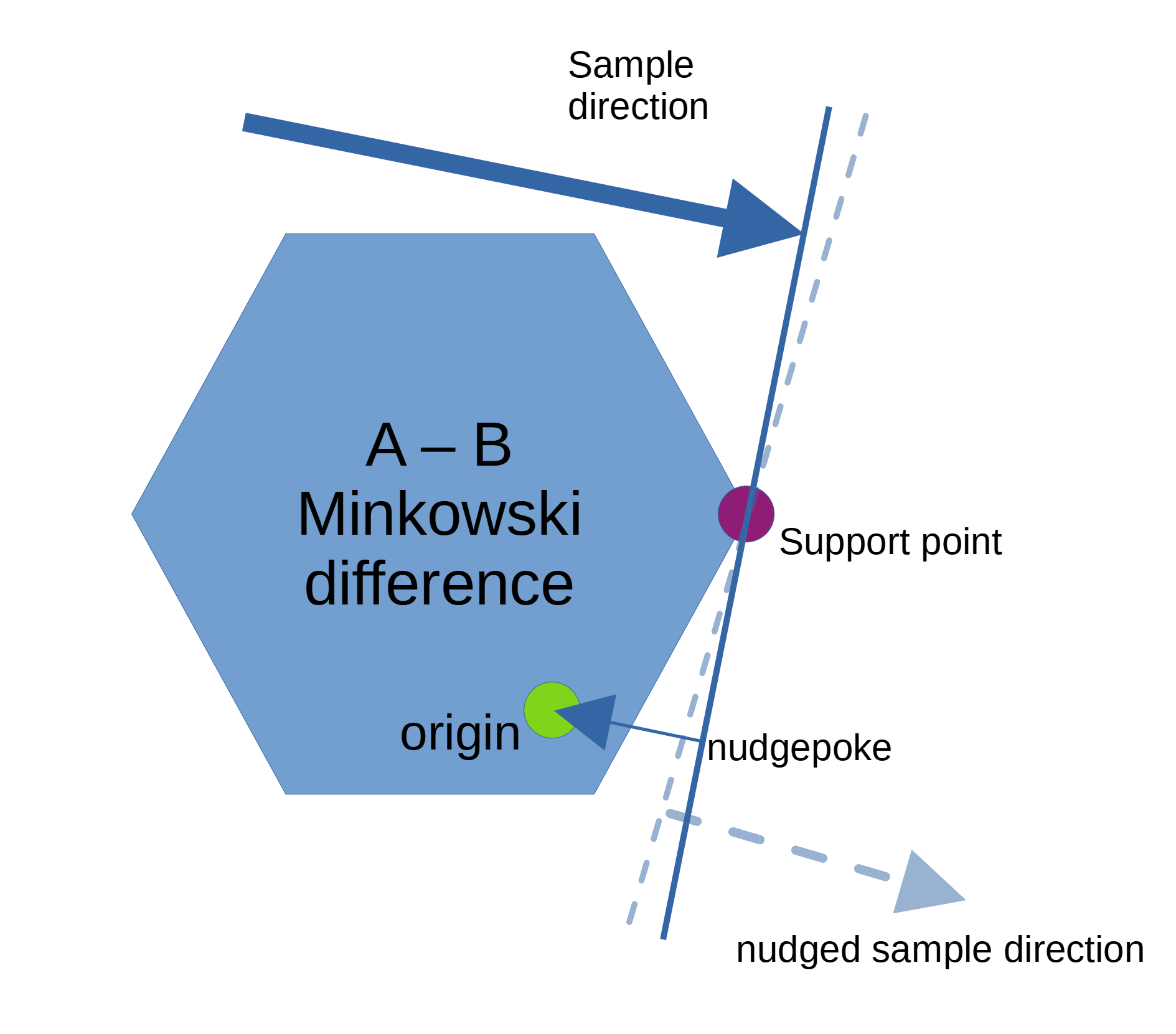
A simple update rule: incrementally tilt the support plane towards the minkowski origin. But how hard do you poke the plane? Too hard, and the plane will tilt past the local minimum and you can end up oscillating or fully diverging. Too gentle, and convergence will take forever.

I fiddled with this a bit. Any time depth increased, it was considered an overshoot and the search would take a half step back, repeating until it got to a point that was better than the pre-overshoot sample. Further, it would reduce the future step size attempt under the assumption that the goal was near. The step size was allowed to grow a little if no overshoot was observed.

It worked reasonably well, but there's a bit of a discontinuity when the support plane goes past the origin. At first, I just did some janky special casing, but it was a bit gross.

A newt looks at me. I feel like I’m missing something obvious.

The Tootbird Dances Furtively

After some further scribbling, I realized I had been a bit of a doof.

There was no need to conditionally 'push' or 'pull' the plane based on the origin's position relative to the support plane. The sample direction simply needed to move toward the origin projected onto the support plane.

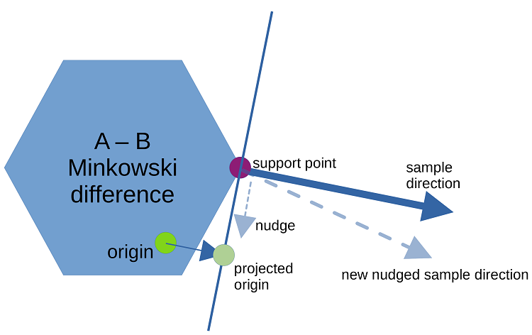
The implementation, dubbed PlaneWalker, used multiple termination conditions: sufficiently small incremental changes to the best observed plane did not find depth improvements, the support point is perfectly lined up with the origin + supportDirection * depth, the discovered depth is lower than the minimum depth (that is, sufficiently negative that the implied separation is larger than the speculative margin), or the maximum iteration count has been reached.

This basic approach actually worked surprisingly well for smooth surfaces, where it tended to significantly outperform GJK and MPR by having a similar iteration count but much simpler individual iterations. This yielded a degree of stokedness.

I experimented with different kinds of history tracking- for example, using the closest point to the origin on the line segment connecting the current overshooting support to the previous support as a guess for the next direction. It helped a bit.

Unfortunately, when the minimal depth direction is associated with a flat surface, plane tilting tends to oscillate back and forth over the surface normal. It still converges by taking progressively smaller steps, but most shapes have flat surfaces, and flat surfaces are very frequently the support feature of minimum depth. GJK and MPR, in contrast, tend to handle polytopes extremely easily. They can sometimes converge to an answer in just a few iterations even without warm starting.

(Even though I didn't end up using the PlaneWalker for any of the current collision pairs, it still works well enough that I suspect I'll find uses for something like it later. It also happens to generalize to higher dimensions trivially...)

The Tootbird Rises

Further scribbling. I tried out a SimplexWalker that extended the PlaneWalker history tracking, which didn't sometimes kinda-sorta helped, but not proportional to the added complexity. I experimented with something that ended up looking like MPR's portal discovery phase (if you squinted) using the projected origin as a dynamic goal, which worked, but the simplex update I was using didn't work in the separating case.

So I began fiddling again with another simplex update rule. Something a bit more GJK-ish- taking the closest point on the existing simplex to a search target... but what search target? Chasing the origin projected on the current support plane is unstable without strong constraints on what support planes are picked- the search target must provably avoid cycles, or else the simplex will never catch it. Using the origin as a search target avoids this issue; that's what GJK does. But finding the origin within the Minkowski difference tells you little about how separate those shapes. So... what search target is immune to cycles, and when sought, finds a local minimum...?

And here, the complete and True Tootbird cast aside the veil and revealed itself: the Minkowski space origin projected onto the least-depth-so-far-observed support plane.

The tootbird could potentially move every iteration. If a support sample found a lesser depth, the tootbird would jump to the new location. Since the tootbird only updates to a lesser depth, chasing it will never cause you to run in circles indefinitely.

Thus, a Tootbird Search is a member of the family of algorithms which incrementally seek the tootbird. Note that the earlier PlaneWalker is technically not a tootbird search, since its objective was always the origin projected on the current support plane even though it did cache the best support plane for backtracking. (It would be pretty simple to make a PlaneWalker variant that was a tootbird search...)

A sample progression of tootbirds with a questionable update rule.

The bepuphysics2 DepthRefiner puts this together with a GJK-style simplex update, yielding a very potent optimizer. A version of the DepthRefiner implementing a 2D tootbird search would look like this:

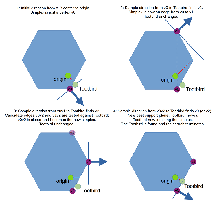
Notice that the simplex in the 2D case never contains more than 2 vertices at one time. The tootbird, by virtue of being on the best-observed support plane, is always outside the Minkowski difference. At most, the simplex can touch the tootbird, but the tootbird cannot be contained. There's no need for the simplex to cover an area (or a volume, in 3D). Further, while we do want to choose the closest simplex when a new sample offers a choice, there is no need to explicitly calculate distances for all candidate simplices. For example, in the 2D case:

Conceptually, it's just a plane test.

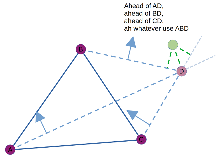
The only significant thing that changes when moving to 3D is that the simplex can become a triangle, and a step can require figuring out which of three potential triangles is the best choice. As in 2D, there's no need to calculate the actual distance for every candidate.

Create edges between the existing vertices A, B, and C and the step's new sample point D. Create a plane for each edge and check which side of the plane the tootbird is on. Based on the signs of the plane tests, you can know which subtriangle (BCD, CAD, or ABD) should be used as the next simplex. This is most clearly visible when D's projection along ABC's normal onto ABC is within ABC:

When D is outside ABC, things are a bit muddier and it's possible for the tootbird to not fall cleanly into any subtriangle by plane tests. This is a pretty rare circumstance, and my implementation shrugs and just takes ABD arbitrarily. This won't cause cycles; the tootbird only changes when a depth improvement is found, so even if our next simplex is a poor choice, it will have a path to march towards the tootbird and possibly improve upon it. You could do something more clever if you'd like.

Once a subtriangle is chosen, the closest offset from triangle to tootbird gives us our next search direction, similar to GJK except with the tootbird as the target rather than the origin.

(My implementation currently has one case where it doesn't use the raw offset as a search direction: when the tootbird is very close to but outside the simplex, the search direction can end up pointing about 90 degrees off of a previous search direction. In some cases, I found this to slow down convergence a bit, so I included a fallback that instead nudges the search direction toward the offset direction rather than taking the offset direction directly. This is similar in concept to the plane tilting described earlier. I'm on the fence on whether this is actually worth doing; the measured impact is pretty minimal, and there are cases where doing the fallback can slow down convergence.)

Drawing full execution diagrams for the 3D version is harder, but there is technically a debug visualizer in the demos. It visualizes the Minkowski difference explicitly through sampling and shows the progress of the simplex for each step. Unfortunately, the interior of flat surfaces on the Minkowski difference are never sampled, so the visualization requires some getting used to. But it's there if you want to play with it!

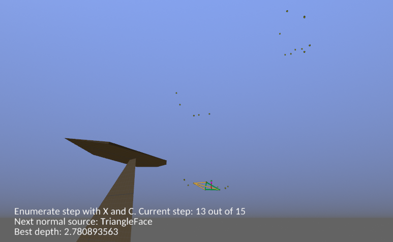
1. In DepthRefiner.tt, set the debug flag to true in the template code,
2. Uncomment the DepthRefinerTestDemo.cs,
3. Add DepthRefinerTestDemo to the DemoSet options,
4. Then try to visually parse this. Or not.

The DepthRefiner implementation terminates when the tootbird is touched by the simplex. A maximum iteration count in the outer loop also helps avoid numerical corner cases.

Notably, once a separating axis is identified (any support direction with a negative measured overlap), a tootbird search could fall back to seeking the origin. The DepthRefiner implementation keeps things simple and sticks to the tootbird at the moment, but depending on the implementation and pair being tested, having a special case for this might be worth it. It would require modifying the termination condition as well.

Further, there's nothing about tootbird search that requires a GJK-ish simplex update. It's just simple and fast. If you squint your eyes a bit, there's also a similarity between the described simplex update and MPR's portal refinement. I'd bet there are some other simplex updates floating out there that would work well with the guarantees provided by the tootbird, too!

Algorithm Extensions

The DepthRefiner tootbird search shares many properties of other Minkowski space collision detection methods. For example, in bepuphysics2, some collision pairs use an implementation which tracks the per-shape contributions to the Minkowski space support point (sometimes termed 'witnesses'). When the algorithm terminates, these witness points along with their barycentric weights corresponding to the closest point on the simplex at termination allow the closest point on shape A to be reconstructed. This is commonly done in other methods like MPR and GJK.

Warm starting is also an important piece of many Minkowski space methods. With a good guess at the initial simplex or search direction, the number of iterations required can drop significantly. Bepuphysics2's implementation of tootbird search does not currently do this, though it is on the to do list and the algorithm itself is compatible with warm starting.

Be careful with warm starting; the algorithm is not guaranteed to converge to a global minimum in all cases. Starting the search process with a bad guess (for example, the direction pointing from the origin to the Minkowski difference's center, rather than from the center to the origin) can easily result in the search converging to a bad local minimum.

Notes on Vectorization

The implementation within bepuphysics2 processes multiple collision pairs simultaneously across SIMD lanes. As a result, performance considerations are similar to GPU shaders: execution divergence and data divergence are the enemy.

To avoid too many conditional paths, the implementation tries to simplify and unify control flow. For example, thanks to the relatively low cost of the worst case simplex update, every single iteration executes the same set of instructions that assume the worst case triangular simplex. When the simplex is actually a point or edge, the empty slots are filled out with copies, yielding a degenerate triangle.

The implementation still contains conditions, but not as many as a fully sequential implementation could take advantage of. The main loop will continue to run until every lane completes. Given that execution batches share the same involved shape types, the number of required iterations is often similar, but this is another area where a sequential implementation would be able to extract more some value. Overall, the widely vectorized version with 256 bit vectors still usually has an advantage, but a sequential narrow vectorization (that is, trying to accelerate only one collision pair as much as possible, rather than doing N pairs quickly) should still be very quick.

For shapes with implicit support functions, like cylinders, support function vectorization is trivial. Data driven types like convex hulls require more work. A vector bundle of shapes could contain hulls with different numbers of vertices, so vectorizing over shapes would require an expensive gather/transpose step and have to always run worst-case-across-bundle enumerations. Convex hulls instead preprocess their internal representation into an AOSOA format and bundle support functions evaluate each shape independently. The support function outputs are transposed back into vector bundles for use by the outer loop.

For readers unfamiliar with modern C# wondering how SIMD is used, in the DepthRefiner it's predominantly through the Vector<T> API. Vector<T> holds a SIMD vector of runtime/architecture defined length. On an old machine limited to SSE42, it could hold 4 single precision floats. On an AVX2 machine, it'll be 8 single precision floats. When the DepthRefiner was written, this (along with types like Vector4) was the main way to take advantage of SIMD in C#. The (compile time) variable width and cross platform requirement meant that many operations were not directly exposed. Shuffles, for example, were a challenge.

In the short time since then, access to vectorization has improved significantly. Hardware specific intrinsics give you the lowest level operations available. More recently (.NET 7 previews), convenience APIs on the fixed-width Vector256<T> and friends are providing the best of both worlds- readable code with high performance that works across multiple architectures. Bepuphysics2 has already adopted the lower level intrinsics in a few hot paths, and there are areas in the DepthRefiner where they'd be useful but are not yet included.

In other words, the DepthRefiner is already a bit old at this point. Some of the implementation choices were dictated by a lack of time, or what options were available. Don't assume that the implementation as-is is the fastest it can possibly be, and feel free to experiment.

Convergence

Given a static tootbird (and leaving aside the current implementation's more complex fallback search direction nudge), the simplex update has the same convergence behavior as GJK when the origin is outside the minkowski difference.

During execution, the tootbird can move, but only if an improvement to depth has been found. It cannot cycle back to higher depth. Since depth is monotonically decreasing over execution, the tootbird will eventually settle into a local or global minimum. At that point, it can be treated as static, and the convergence properties of GJK apply.

In practice, the simplex and tootbird move rapidly together and settle on a local minimum quickly. The number of iterations required is similar to GJK in my experiments. The per-step cost is lower, given the guarantees provided by the tootbird being outside of the Minkowski difference. I would expect the performance to be similar and depend on details of implementation and use case.

So, empirically, does it work, and is it fast enough?

Yup!

FAQ

Q: okay but why is it called tootbird

A: what do you mean

bepuphysics v2.4.0 released!

It’s way faster! Github!

bepuphysics v2.3.0 released!

Grab: https://github.com/bepu/bepuphysics2/releases/tag/v2.3.0

Moving to github discussions

I’ve put the phpBB forums into read only mode; for future discussions and questions, please use the repository discussion tabs!

v1: https://github.com/bepu/bepuphysics1/discussions
v2: https://github.com/bepu/bepuphysics2/discussions

Also, since I haven’t announced it here yet- note that nuget prerelease packages are now released automatically. If you are still using 2.2.0, consider updating to the newer 2.3.0 betas (or whatever is out when you read this)!

v2.2.0 released!

I figured rather than waiting another year for a nuget release, I’d try a slightly more frequent release cadence.

On Github
On NuGet

v2.1 released, discord experiments

Bepuphysics v2.1 has been released and pushed out to nuget packages. It includes all the accumulated changes since release- nothing groundbreaking, but lots of small improvements, convenience features, and bug fixes.

At the request of some users, I’ve also created a discord as an experiment. I will still focus on the forum/github for long-form content, but I will pop in occasionally.

Give me your dollars on GitHub Sponsors!

I’ve recently been accepted to the GitHub Sponsors program!

I’ve fancied up the support tiers and added a newt-themed SponsorsDemo, among other somewhat more professional rewards like private email support and poorly drawn animals. Due to the lower fees and matching, I recommend github sponsors over patreon, but the patreon will stick around for a while.

Head over to my sponsors page to give me money!

bepuphysics v2 is out of beta!

Get yourself some blazing fast physics on github!

(🔥)

... but GPUs aren't always the right choice

In the last post, the fictional Toilet Toilers Interactive found themselves in a bit of a pickle with their GPU physics-and-everything-else pipeline. They might be regretting some of their technical choices, but it’s worth looking back at some of the things they might have considered during development. Why might they have decided to walk such an unusual path, and why didn’t bepuphysics v2?

GPUs are indeed fast

Bepuphysics v2 is primarily sensitive to two architectural details: memory bandwidth and floating point throughput. Moving from a quad core 4-wide SIMD CPU with dual channel DDR3 memory like the 3770K to a 7700K with AVX2 and higher clocked DDR4 can give you huge speedups. That’s despite the fact that it’s still just a quad core and the general purpose IPC/clock improvements from Ivy Bridge to Kaby Lake aren’t exactly groundbreaking.

Suppose we wanted to go crazy, and suppose I also managed to address some potential scheduling issues on high core count systems. AMD’s EPYC 7601 could be a good choice. Even though Zen 1 doesn’t have the same per-core floating point throughput as contemporary Intel CPUs or Zen 2, the massive number of cores enable a respectable 600+ gflops. With 8 memory channels of DDR4 memory, you can pretty easily hit 3 to 4 times more effective memory bandwidth than a 7700K (120+ GBps).

Now consider a high end graphics card. The 7601 is on the premium end of the pricing spectrum, so we’ll look at a 2080 TI: 13.4 tflops and 616 GBps memory bandwidth. The Radeon Instinct MI60 (with a large chunk of HBM2) has about 1 TBps bandwidth.

Even if you drop the budget into more reasonable territory, the gap between CPU and GPU persists. Graphics cards are simply designed for massive throughput and are ideal for highly parallel workloads that can make use of their extremely wide hardware.

Graphics are clearly a perfect fit for graphics hardware, but graphics cards have become progressively more general in their capabilities. We’ve moved from fixed function transforms up to a level of generality spanning cryptocurrency mining, protein folding, ray tracing, and yes, physics simulation.

So, if the Toilet Toilers thought they could get such a huge benefit by embracing GPU execution fully, why would I build bepuphysics v2 for the CPU?

Algorithms and architectures

Achieving decent multithreaded scaling generally involves phrasing the computation as a giant for loop where every iteration is independent of the others. Bonus points if you can guarantee that every iteration is doing the exact same type of work, just on different data. This applies to both CPUs and GPUs, but GPUs will tend to massively outperform CPUs in this use case.

Case study: collision batching

We don’t always have the luxury of doing the exact same type of independent task a million times. Consider the narrow phase of collision detection. In bepuphysics v2, each worker generates an unpredictable stream of collision pairs. The type, number and order of the pairs are not known ahead of time. This introduces some complexity. One potential GPU implementation would be to have a pass dedicated to extracting all the jobs from the collision pair stream and adding them to big contiguous lists. After the pass completed, you’d have the list of every sphere-sphere pair in one spot, every sphere-capsule in another spot, and so on. It could look something like this:

You could then dispatch the appropriate collision handler for each pair type. With a sufficient number of pairs, the GPU would achieve a decent level of occupancy.

But there remain some concerns. On the GPU, you’ve got potentially thousands of workers. Are you going to write a single shared set of type batches with global atomic counters? And you spent all that time writing everything in the first pass, only to then go back and read it all again in the second pass- that’s a lot of memory bandwidth used!

You’re not yet out of options, but now things start getting more complicated. Maybe you could create an intermediate set of type batches that accumulates a small local set in thread group shared memory that gets flushed to the main set only periodically, cutting down the number of global atomic calls. Maybe you do something clever with wave operations.

But even if the bookkeeping costs aren’t a concern, the theoretically pointless write-then-read issue is still there. Maybe you could take advantage of some features that are implied by hardware accelerated ray tracing. Ray tracing with unpredictable target surface shaders is actually a very similar problem, and as hardware adapts to support ‘callable shaders’ efficiently, options could open.

In CPU-land, we can just stick each pair into a thread local type batch. When the type batch count reaches some execution threshold- say, 16 or 32 entries- flush it. In most cases, that means the data in the type batch is still in L1 cache, and failing that, it will almost always still be in L2 cache. Swapping tasks from pair collection to executing the pair processor for a type batch does carry some overhead, but for a CPU, we’re talking about a few dozen nanoseconds on the high end. That doesn’t really matter when the execution of the type batch is expected to take a handful of microseconds.

As the workarounds showed, implementing something similar on a GPU is not fundamentally impossible, but it’s not natural for the device and you probably won’t be achieving that 13.4 teraflops number with a bunch of code like this (at least for a while). At a high level, CPUs are latency optimized and handle these sorts of small scale decisions easily, while GPUs are throughput optimized. That focus is reflected across the hardware, tooling, and programming model; going against the grain is uncomfortable.

Case study: dynamic hierarchy broad phase collision testing

Algorithms vary in their parallelizability. Some are stubbornly resistant to any kind of multithreading, others require a bit of effort to tease out the parallelism, and others are just embarassingly parallel. In many cases, when there exist sequential and parallel algorithms for the same task, the more sequential version has a significant advantage that can only be overcome by throwing quite a bit of hardware at the parallel version.

Bepuphysics v2’s broad phase contains an interesting example of this phenomenon. It uses a dynamically updated binary tree. To find out which collision pairs exist, all leaves of this tree must somehow be tested against the tree.

The naive algorithm is very simple and is a decent fit for a GPU or other very wide machine: loop over every collidable and test its bounding box against the tree. Every test is completely independent.

But note that we’re loading the tree’s nodes over and over again. The whole tree could be multiple megabytes, so tiny core-local caches won’t be able to serve most requests. Even without the extra cost of hitting more distant caches or main memory, that’s still a lot of bounding box tests. As always, there are some potential optimizations or workarounds, and as usual, they come with some complexity penalties.

There exists a very simple algorithm that avoids the need for most of this work. Consider two separate bounding trees- test the roots against each other; if they intersect, test all combinations of their children (for pair of binary trees, childA0-childA1, childA0-childB1, childB0-childA1, childB0-childB1); for the pairs that intersect, recursively continue the same process. The result is all overlaps between leaves in tree A and tree B.

Now, we can go one step further: run that same process, except between a tree and itself. Note that there’s no need to do many of the intersection tests because any node obviously overlaps with itself. Not only has the number of intersection tests dropped considerably compared to the naive approach, but we’ve also eliminated all the redundant node loads.

This algorithm is not horribly sequential- it spawns independent work recursively- but it’s not embarassingly parallel either. In other words, if you’ve got 64 fat cores, you can create enough worker tasks to fill the hardware cheaply. But, if your target architecture has many thousands of very weak threads, suddenly the setup work is significant.

(It’s worth mentioning that ‘threads’ exposed by graphics APIs aren’t mapping to the same sort of thread as you get on an x86 CPU. They’re more like lanes in wide SIMD units. You can take advantage of this sometimes, but again, going against the grain comes with a complexity penalty.)

So what does all this mean? To naturally fit a GPU, you’ll generally want to pick algorithms that suit its execution style. Sometimes this means paying an algorithmic penalty to use a more parallel implementation. In these cases, you sacrifice some of that crazy compute power in order to use it at all.

Of course, even a handicapped GPU can still beat a CPU sometimes.

Case study: bookkeeping

The least exciting parts of a simulation can sometimes be the hardest to bring over to extremely wide hardware. Consider the process of adding constraints to the solver based on collision detection results. Every constraint addition requires multiple sequential steps and separating them into even somewhat parallel tasks involves terrible complexity.

Each new constraint must identify a solver batch that does not share any bodies with the new constraint, then it must find (and possibly create or resize!) a type batch for the new constraint to belong in. And then it has to reach into the per-body constraint lists to ensure a traversable constraint graph. And so on. It’s tied for my least favorite part of the engine, and it’s all because I attempted to extract parallelism where there was very little available.

And then you have even more fun things like sleeping and waking. Beyond merely adding a bunch of constraints and updating all the related bodies to match, it also moves a bunch of bodies and updates the broad phase at the same time. (I’d link a bunch of stuff related to it, but I can’t be bothered to go find all the tendrils.)

Even with all that effort, the scaling is still pretty bad. Especially sleep/wake which bottlenecks badly on the broad phase modifications. I aim to improve that at some point, but I really, really don’t look forward to it. On the upside, our big fat latency optimized CPUs still do reasonably well. Bookkeeping is rarely a noticeable fraction of frame time unless you happen to be sleeping a 16000-body pile.

Without the benefit of big x86 cores to brute force through these locally sequential chunks, this work could become a serious problem. Trying to do all of this work on a few GPU ‘threads’ (in the HLSL sense of the word) is a nonstarter. Realistically, it would require a completely different approach to storage- or punting the work to a fatter core. It wouldn’t be enjoyable in any case.

The pain of asynchrony

Any time your simulation is executing out of step with some interacting system (like game logic), a blob of complexity is introduced. All interactions between the systems must be carefully managed. This applies to asynchronous use on both the CPU and GPU, but running a simulation on the GPU will tend to imply a thicker barrier. Even merely moving data across PCIe takes extra time.

Game logic often benefits from fairly tight integration with the simulation. Writing a callback that can modify the simulation state or report data on the fly gets a lot harder if that callback needs to execute on the GPU. In practice, a whole lot of simulation state will only be indirectly accessible. You can definitely still work with it, but everything gets a little bit harder.

There’s also the option of embracing it entirely like the Toilet Toilers did- execute even most of game logic on the GPUs. I might call you nuts, but you could do that. The helpfulness, speed, and stability of tools in GPU land typically struggle to meet the expectations you might have from working in CPU land…

All the asynchronous pain disappears if the only consumer of your simulation is graphics and your graphics and simulation are synchronized. Noninteractive debris, many forms of cloth, particles and other decorative simulations are great use cases for GPU physics that avoid asynchrony’s suffering entirely. That just wasn’t my target use case for bepuphysics v2.

Comparative advantage

In many games, all the crazy horsepower that a GPU brings to the table is already spoken for. Rendering 4K@120hz with ray traced global illumination is still beyond all current hardware, and by the time we have the hardware for it, we’ll be trying to render dense lightfields for VR or something.

Is it worth turning down some of that graphical fanciness to run physics? If we assume that a GPU implementation is 4 times faster and that all the concerns above are dealt with, we could move a 6 millisecond CPU simulation to the GPU for a mere 1.5 milliseconds. If the simulation and rendering are both targeting 144hz, then you’ve cut your rendering budget by 20%, but massively increased your CPU budget! … now what are you going to do with that CPU budget?

You could waste a bunch more time in the driver by spamming draw calls, I suppose. You could generate a wonderful number of draw calls with DX12 or Vulkan and multiple threads. Or you could use indirect rendering and a gpu driven pipeline…

Maybe you could do some fancy sound tracing and dynamic audio effects! But a lot of the queries would fit the simulation structures really well, and pulling that across PCIe every frame seems wasteful, and the actual math involved would fit the GPU…

Or maybe use some fancy machine learning techniques to animate your characters, but then GPUs (especially ones with dedicated hardware for it) do inference way faster than CPUs…

I don’t mean to imply that there’s nothing you could spend that CPU time on, just that a lot of heavy lifting does map well to the GPU. Despite that, there’s no point in leaving the CPU idle. It makes sense to give the CPU work that it can do reasonably well, even if the GPU could technically do it faster- because the GPU is doing something else already!

(Backend use cases can be interesting- the lack of rendering on the server could open up space for many more jobs. You’d still suffer from many of the other issues listed here, but at least you’d have the computational resources freed up.)

The deciding factor

I’ve gone through a variety of concerns with GPU simulations, but I’ve also tried to offer some workarounds in each case. It’s definitely possible to make a speedy GPU simulation- it has been done, after all.

But there’s one problem that I can’t find a way around. Making a complex GPU-heavy application run reliably across different hardware vendors, hardware generations, operating systems, and driver versions is extremely painful. Past a certain level of complexity, I’m not actually convinced that it’s possible without having a direct line to all the involved engineering teams and a few metric hecktons of dollars. I do not have that many dollars, and not many people know I exist; hitting a particularly dangerous driver bug can kill an entire line of research.

And, even if I manage to achieve a reasonable level of stability somehow, regressions in newer drivers- especially on older hardware- are not uncommon. The fate of the Toilet Toilers was only slightly exaggerated, and only in terms of temporal density.

I can try to report all the issues to all the different parties involved, but honestly, I can’t blame them if they don’t fix a problem even 5 years later. Some of these problems are just weird little corner cases. Some of them don’t apply to any modern hardware. It makes perfect sense to spend limited development resources on the projects that are actually going to drive many millions or billions of dollars in sales. (Maybe one day!)

You might notice that this line of thinking almost suggests that any GPU development is a lost cause for a small player, not just GPU physics. As frustrating as the ecosystem is, I’m not willing to go that far. There are a few important distinctions between graphics and physics.

In a physics simulation, the result of one time step feeds into the next, and into the next, and so on. If any stage fails at any point, it can cause the entire simulation to fail. For example, a single NaN will propagate through a constraint graph within a frame or two. Within another frame or two, the simulation will probably crash.

Graphics tend to be slightly more resilient. There are still types of bugs which can bring everything crashing down, certainly, but most of the milder bugs can be survived. They might just result in a bit of visual corruption here or there- once it’s out of any temporal accumulation windows, the problem may resolve.

In other words, in graphics-like tasks, data dependency chains tend to be short. Error does not have a chance to feed upon itself catastrophically, or the error is bounded.

Further, graphics engines often have lots of tuning knobs or multiple implementations of effects for different quality levels. Bugs can sometimes be worked around by fiddling with these knobs. Physics simulators usually don’t have as many degrees of freedom.

Finally, if you are working on graphics as a smaller developer, chances are you’re targeting just one API and operating system. Focusing on, say, DX12 on Win10 alone won’t be easy, but it’s not the nightmare that supporting other operating systems/APIs simultaneously would be. (The same can be said for some client-only GPU physics use cases, but if you want to run physics serverside, it’ll probably need to run on things that aren’t windows- because the server licensing model is the only thing worse than driver bugs.)

But even for graphics, the situation is nasty enough that using one of the super popular graphics engines is wise if you intend to target a variety of platforms. It’s a well-worn path that a thousand other developers have walked already; they have suffered for you.

Conclusion

If I built bepuphysics v2 to run on the GPU, I could probably make it faster. It would take a long time and I’d want to gouge out my eyes at many points during the process, but I could do it.

It wouldn’t match up with how I want to integrate it into other projects, and I have other things I can spend those GPU cycles on.

Plus, v2 performance already approaches (and occasionally exceeds) some GPU rigid body simulators, so I’m pretty okay with it.

GPUs are fast...

August 23, 2019, 2:23 PM

You are one of the four founding members of Toilet Toilers Interactive, a development studio riding a wave of popularity after a successful paid alpha launch.

Punching and Whatnot, your genre-fusing open world exploration game about physically punching things, attracted an early and devoted audience on the promise of its marketed-as-revolutionary technology stack.

Development videos of many thousands of punchings simulated in real time spread virally through the latest and most confusing forms of social media.

Critics hail your game as 'much better than it sounds'. Development costs have largely been recouped.

Your team, a group of technological pioneers in the field of simulated pugnacity, have the attention of the gaming world.

And this is your job.

"It's really not that hard, you just gotta..." you say, carefully manipulating a plate covered in crumbs.

"You're using your thumb," says your cofounder Minji, leaning back in a chair across from you with her arms crossed in skepticism.

"No I'm not," you say, putting the plate back down on the desk.

"Yes you were, I saw it."

"It was touching, but the thumb was barely even acting as a stabilizer."

"A person without thumbs doesn't get to use their thumbs as barely-stabilizers. Do it again, no thumb."

"Fine," you huff, making a show of extending your thumb as far as possible before grabbing the plate between your forefingers. Your phone vibrates, but this task demands your whole focus.

Minji waits.

The plate rises, slowly, carefully... and your phone vibrates again.

Loud obscenities ring through the office, grabbing Minji's attention. You quickly let the plate down, sending a few unstuck mealsquare crumbs onto your desk.

"See, it's easy," you begin, but are interrupted by the sound of rapid British-sounding footsteps approaching the doorway.

"ALL THE SERVERS ARE DOWN!"

August 23, 2019, 3:13 PM

You are all quite proud of the infrastructure you've built. Almost everything that could be automated, is. Need to update the servers? Zero downtime rolling automated installs. Crashes or hardware failure? Automatic load balancing fills in the gap as needed. Want to check server status? Fancy graphs on your phone.

All without using any off the shelf technologies. Everything from scratch. (It added 15 months to the project, which, as you frequently tell yourself, isn't really that long and it was definitely probably worth it.)

And, as a testament to just how robust it all is, it took three whole weeks after release to hit your first catastrophic failure and multi-hour outage.

"The servers are up on the previous deployment. Backups were untouched, all data retained," Minji says from across the conference table.

You smile smugly, nodding to yourself. The backup system had been your baby. To your right, Geir (whose name is pronounced something like Guy, but who asserts that you are still saying it wrong, but that's his fault for having such a British name) notices your self-satisfaction and gives you a look which you take as affirmation of your work's quality.

"Nominal levels of forum angst. I don't think we'll have to do more than offer a brief explanation," adds Kazimiera from your left, who had settled into a sort-of-community-manager role in addition to the rest of her regular developmental responsibilities.

"So, unless someone else snuck something into that last image, the only change was a new graphics driver. There's a new WHQL release that apparently fixed some of the tiled resource slowdowns we had to work around. I put it on the test servers and it came back all green," Geir said.

You furrow your brow. Kazimiera types furiously on her laptop.

"I thought we fixed that -" you begin, vague memories mixing with rising unease in your stomach.

"All test servers are dead," says Kazimiera.

"We didn't fix that."

You lean back in your chair.

"So, it's possible that we may have forgotten to address a small issue wherein the tests can sometimes, under complex conditions involving driver freezes, time out and return success, instead of not success," you explain to Geir, who had missed the fun. He squints at you.

"How does the tech support forum look?" asks Minji.

Kazimiera clicks around.

"A couple of 'server down' posts... Oh, someone is actually playing on integrated, and it's working! Except all skinned characters have little flickering black dots at every vertex."

"As it should be," says Minji, nodding.

"And about four 'help my game is completely broken' in the last few days, which is two or three more than usual."

"It went WHQL a few days ago," offers Geir.

Everyone sits quietly for a moment, staring into space.

"Alright," starts Minji, slapping the table. "It looks like we need some proactive action, I'm gonna be the scrummer. The scrum lord. It's time to get agile."

"But are you a certified scrum lord?" you ask.

"Kazi, kindly draw us a burndown chart," she says, ignoring you.

Kazimiera gets up and walks toward the whiteboard.

"British graphics expert," she says, pointing at the sighing Geir. "The surface space allocator uses sparse textures right? Would you confirm that everything is broken on the client?"

Geir nods.

Kazimiera is finishing up the labels on her chart. A line starts in the upper left and heads to the lower right, carefully dodging an older drawing of a cat. The line spikes upward to a point above the starting height a few times. The horizontal axis is labelled TIME, and the vertical axis CATASTROPHIC BUGS.

"Thank you, Kazi. I feel adequately scrummed. I'd like your help actually-fixing the test harness. And we should probably post some warnings."

Kazimiera caps her marker and returns to her seat.

Minji turns to you.

"There aren't a lot of GPU jobs on the backend, and you happen to have written all of them," she says.

You make a small noise of acknowledgement tinged by indignity.

August 23, 2019, 5:56 PM

The backend physics was, in fact, not working on the new driver version. Your workstation's card, a slightly older generation with an architecture named after a different dead scientist, exhibits the same problem. The reference device works fine.

With some effort and bisection, you've gotten to the point where things do not instantly crash. On the downside, the only active stage remaining is a single piece of the broad phase pair flush. And, given dummy input, it's producing nonsense results.

You launch the program again with a VS capture running, and it immediately crashes.

Pursing your lips, you start up NTRIGUE, a vendor created tool that was recently rebranded for unclear reasons. It looks like it's working, but starting a frame capture immediately crashes.

You take a deep breath and exhale slowly.

August 26, 2019, 1:52 PM

"As scrum lord, I hereby convene this scrummoot. Geir, care to begin?"

"Lots of things are busted. For example, with anisotropic filtering x8 or higher enabled, while indexing descriptor arrays in the pixel shader, in the presence of sufficiently steep slopes at over one hundred kilometers from the camera, the device hangs. I am not yet sure how to narrow down the repro further. Also I'm not sure if tiled resources should be considered to exist anymore."

"Sounds good. And the physics?" Minji asks, looking at you.

"I fixed a bug!"

"Care to elaborate?"

"Mm, no."

Kazimeria clicks a few times. "Group memory barriers added to a parallel reduction. Something something shouldn't be necessary, something something memory writes in thread groups below hardware threshold should proceed in order, but added them anyway."

Geir gives you a look.

"Does everything work now?' asks Minji.

"Mmmmm, no."

Kazimiera clicks a few more times. "Only one dispatch is actually completing without hanging the device," she explains. "Your commit descriptions are admirably thorough. Except this one of an ascii butt."

"On the upside, we should have the test suite fixed today or tomorrow," says Minji.

"Content pipeline's fine, by the way. Auto-animation net is still working flawlessly," adds Kazimiera.

"The Demon Prince of Drivers is patient," you warn.

August 27, 2019, 2:40 PM

You slump into your chair. Geir, arriving sooner, has already slid far enough down that only his shoulders and head are visible above the conference table.

"Praise be to scrum," chants Minji.

"My turn to start," you say. "FFFfffffffffffffffffffffffffffffffffffffffffffffffffffffffffffffffffffffffffffffffffffffffffffff," continuing until you run out of breath.

"How many points is that so I can mark it in my scrumbook?"

"...Seven...teen."

"I 'fixed' the terrain thing by detecting the vendor hardware and clamping maximum render distance. I submitted a bug report, but the repro sucks. Also, there's still some other bug where root sampler state gets corrupted- previous data gets reused, stuff explodes." says Geir.

"Good work, I award you one thousand points."

"That's no fair!" you whine.

"Well, have you submitted any bug reports yet?"

"Do you think they would fix it if I just submit a bug report that is the sound of frustrated yelling?" you ask, sliding down your chair a little.

"That may be a significant fraction of the total reports, you should put in some more effort so it will get noticed. Maybe try yelling louder," offers Kazimiera.

"That's a promising idea," you say, rubbing your chin. "Alright, well, under some conditions I have not yet narrowed down, UAV barriers seem to do nothing, and the physics is a series of compute dispatches, so, hooray. For clients, I may be able to work around it by forcing some sort of useless transition or other stall. But it will be a pretty big performance hit and there's not enough headroom for it to be used on the backend, so we can't update the drivers there."

"Interesting. Four more agile points for you. As for me, I've been tracking down some of the non-crashy problems on the client. It looks like all indirect executions now cost a minimum of about max command count times one or two microseconds, regardless of the actual count in the count buffer. I should be able to have that reported today. For this, I earn many points," says Minji.

"And I've just finished a little optimization on the proxy server that cuts minimum latency by half a millisecond," says Kazimiera.

"How does it feel, up in your ivory tower? Frolicking lightly above the clouds, free to make forward progress?" you ask.

Kazimiera smugs.

August 28, 2019, 4:33 PM

"So, I worked around the missing barriers at a slowdown of about four hundred percent," you explain. "To mitigate this slowdown, I propose spending three hundred and fifty thousand dollars on new hardware instead of continuing to work on it because I do not want to work on it."

"Any response from the vendor?" asks Minji.

Kazimiera hits F5. "No."

"Cool, cool, cool, cool, cool, cool, cool, cool, cool," says Minji, tapping a pen against the conference table to match. She sinks sideways, propping herself up with one elbow. "Lord British," she says, pointing the pen at Geir without turning, "tell me what you got."

"Sometimes I wonder if it was a good idea to leave Norway."

"Oh, my aunt went there once! Pretty long drive out, I heard. That's like a hundred miles northeast of London, isn't it?" asks Minji earnestly.

Geir shook his head, badly suppressing a smile.

"You know, we're semifamous now," starts Geir. "And a whole lot of their customers are immersed in our completely broken mess. They will probably be a little more motivated to work with-"

"Um," interrupts Kazimiera.

Everyone looks over.

"Windows 10 Creative Pool Summer Hangout update is rolling out. Staged, but should expect a lot of users to be on it within a week or two. It apparently changes some bits of the graphics stack."

Geir's eyes widen.

"It autoupdates to the latest WHQL driver."

This story is fictional. The bugs are not :(

A different kind of C#: going wide

Writing efficient SIMD-accelerated code can be tricky. Consider a single cross product:

result.X = a.Y * b.Z - a.Z * b.Y;
result.Y = a.Z * b.X - a.X * b.Z;
result.Z = a.X * b.Y - a.Y * b.X;

If you'd like to try a brain teaser, imagine you’ve got subtract, multiply, and lane shuffle operations that can handle 4 lanes of data at the same time. Try to come up with the minimal number of operations needed to express the same mathematical result for a single pair of input 3d vectors.

Then, compare it to the scalar version. Without spoiling much, it's not going to be 4x faster with 4-wide operations.

Problems like this show up any time you try to narrowly vectorize scalar-ish code. You rarely get the benefit of 128 bit operations, let alone newer 256 bit or 512 bit operations. There just aren't enough independent lanes of computation to saturate the machine with real work.

Fortunately, most compute intensive programs involve doing one thing many times to a bunch of instances. If you build your application from the ground up assuming this batch processing model, it doesn’t even involve more difficulty than traditional approaches (though it does have different difficulties).

Let’s assume we’ve got a nice big batch of 2^20 operations to perform, each computing:

result = dot(dot(cross(a, b), a) * b, dot(cross(c, d), c) * d)

Array of Structures

We’ll start with a naive scalar implementation and a narrowly vectorized version as a basis for comparison. They could look something like this:

public struct Vector3AOS
{
  public float X;
  public float Y;
  public float Z;
  ...
}

for (int i = 0; i < LaneCount; ++i)
{
  ref var lane = ref input[i];
  Vector3AOS.CrossScalar(lane.A, lane.B, out var axb);
  Vector3AOS.CrossScalar(lane.C, lane.D, out var cxd);
  var axbDotA = Vector3AOS.DotScalar(axb, lane.A);
  var cxdDotC = Vector3AOS.DotScalar(cxd, lane.C);
  Vector3AOS.ScaleScalar(lane.B, axbDotA, out var left);
  Vector3AOS.ScaleScalar(lane.D, cxdDotC, out var right);
  results[i] = Vector3AOS.DotScalar(left, right);
}

for (int i = 0; i < LaneCount; ++i)
{
  ref var lane = ref input[i];
  Vector3AOS.Cross3ShuffleSSE(lane.A, lane.B, out var axb);
  Vector3AOS.Cross3ShuffleSSE(lane.C, lane.D, out var cxd);
  Vector3AOS.DotSSE(axb, lane.A, out var axbDotA);
  Vector3AOS.DotSSE(cxd, lane.C, out var cxdDotC);
  Vector3AOS.ScaleSSE(lane.B, axbDotA, out var left);
  Vector3AOS.ScaleSSE(lane.D, cxdDotC, out var right);
  Vector3AOS.DotSSE(left, right, out var result);
  results[i] = Sse41.Extract(result, 0);
}

(The full implementation for all of these approaches can be found in the GoingWide project in the scratchpad repo.)

They’re both very similar at the level of memory accesses. Load the relevant whole struct instance from the array (hence array of structures!), do some work with it, store it out. At a lower level, the SSE version is a bit weirder. For example, the Vector3AOS.Cross3ShuffleSSE function is not quite as intuitive as the earlier cross product code:

const byte yzxControl = (3 << 6) | (0 << 4) | (2 << 2) | 1;
var shuffleA = Sse.Shuffle(a, a, yzxControl);
var shuffleB = Sse.Shuffle(b, b, yzxControl);
result = Sse.Subtract(Sse.Multiply(a, shuffleB), Sse.Multiply(b, shuffleA));
result = Sse.Shuffle(result, result, yzxControl);

Only three of those intrinsics calls are actually doing arithmetic.

Despite its ugliness, the SSE variant is faster even with the current alpha state of intrinsics support by about 25-30%. Still a far cry from 4x faster.

To do better than this, we need to make use of the fact that we’re doing the same thing a million times in a row.

Structure of Arrays

Array of structures (AOS) lays out memory instance by instance. Each struct contains all the data associated with one instance. That’s pretty intuitive and convenient, but as we’ve seen, it’s not a natural representation for wide vectorization. At best, you’d have to convert the AOS memory layout into a vectorized form at runtime, perhaps walking through multiple instances and creating vectorized bundles of instance properties. But that takes valuable time that we could be spending on actual computation!

What if we just stored every instance property in its own big array?

Buffer<float> ax, ay, az, bx, by, bz, cx, cy, cz, dx, dy, dz, result;

public override void Execute()
{
  for (int i = 0; i < LaneCount; i += Vector<float>.Count)
  {
    ref var ax = ref Unsafe.As<float, Vector<float>>(ref this.ax[i]);
    ref var ay = ref Unsafe.As<float, Vector<float>>(ref this.ay[i]);
    ref var az = ref Unsafe.As<float, Vector<float>>(ref this.az[i]);
    ref var bx = ref Unsafe.As<float, Vector<float>>(ref this.bx[i]);
    ref var by = ref Unsafe.As<float, Vector<float>>(ref this.by[i]);
    ref var bz = ref Unsafe.As<float, Vector<float>>(ref this.bz[i]);
    ref var cx = ref Unsafe.As<float, Vector<float>>(ref this.cx[i]);
    ref var cy = ref Unsafe.As<float, Vector<float>>(ref this.cy[i]);
    ref var cz = ref Unsafe.As<float, Vector<float>>(ref this.cz[i]);
    ref var dx = ref Unsafe.As<float, Vector<float>>(ref this.dx[i]);
    ref var dy = ref Unsafe.As<float, Vector<float>>(ref this.dy[i]);
    ref var dz = ref Unsafe.As<float, Vector<float>>(ref this.dz[i]);

    Cross(ax, ay, az, bx, by, bz, out var axbx, out var axby, out var axbz);
    Cross(cx, cy, cz, dx, dy, dz, out var cxdx, out var cxdy, out var cxdz);
    Dot(axbx, axby, axbz, ax, ay, az, out var axbDotA);
    Dot(cxdx, cxdy, cxdz, cx, cy, cz, out var cxdDotC);
    Scale(bx, by, bz, axbDotA, out var leftx, out var lefty, out var leftz);
    Scale(bx, by, bz, cxdDotC, out var rightx, out var righty, out var rightz);
    Dot(leftx, lefty, leftz, rightx, righty, rightz, out Unsafe.As<float, Vector<float>>(ref result[i]));
  }
}

(Note that the above implementation is uglier than it needs to be- the goal was to keep it conceptually separated from the next approach, but a real implementation could be less verbose.)

This turns out to be about 2.1x faster than the original scalar version. That’s an improvement, even if not quite as large as we’d like. Memory bandwidth is starting to block some cycles but it’s not the only issue.

One potential concern when using SOA layouts is an excessive number of prefetcher address streams. Keeping track of a bunch of different memory locations can hit bottlenecks in several parts of the memory system even if each access stream is fully sequential. In the above, the 13 active address streams are enough to be noticeable; if expressed in the same kind of SOA layout, the current Hinge constraint would have 47 streams for the projection data alone.

You could also try changing the loop to instead perform each individual operation across all lanes before moving on to the next one (i.e. multiply all ay * bz, store it in a temporary, then do all az * by and store it, and so on). That would indeed eliminate address streams as a concern given that there would only ever be two or three in flight at a time. Unfortunately, every single operation would evict the L1, L2, and with a million instances on many consumer processors, even all of L3. No data reuse is possible and the end result is a massive memory bandwidth bottleneck and about 3.5x worse performance than the naive scalar version. Now consider what it might look like if the loop were modified to process a cache friendly block of properties at a time…

Tying it together: Array Of Structures Of Arrays

We want something that:

1. allows efficient vectorized execution,

2. is usable without SPMD/SIMT tooling (see later section),

3. feels fairly natural to use (preserving scalar-ish logic),

4. is cache friendly without requiring macro-level tiling logic, and

5. doesn't abuse the prefetcher.

There is an option that meets all these requirements: AOSOA, Array Of Structures Of Arrays. Take the bundled Structure Of Arrays layout from earlier, restrict the array lengths to be the size of a single SIMD bundle, shove all of those smaller bundle-arrays into a struct, and store all those bundle-array containing structs in an array. Or, to put it in a less grammatically torturous way:

public unsafe struct Vector3AOSOANumerics
{
  public Vector<float> X;
  public Vector<float> Y;
  public Vector<float> Z;
  ...
}

struct Input
{
  public Vector3AOSOANumerics A;
  public Vector3AOSOANumerics B;
  public Vector3AOSOANumerics C;
  public Vector3AOSOANumerics D;
}

Buffer<Input> input;
Buffer<Vector<float>> results;

public override void Execute()
{
  for (int i = 0; i < LaneCount / Vector<float>.Count; ++i)
  {
    ref var lane = ref input[i];
    Vector3AOSOANumerics.Cross(lane.A, lane.B, out var axb);
    Vector3AOSOANumerics.Cross(lane.C, lane.D, out var cxd);
    Vector3AOSOANumerics.Dot(axb, lane.A, out var axbDotA);
    Vector3AOSOANumerics.Dot(cxd, lane.C, out var cxdDotC);
    Vector3AOSOANumerics.Scale(lane.B, axbDotA, out var left);
    Vector3AOSOANumerics.Scale(lane.D, cxdDotC, out var right);
    Vector3AOSOANumerics.Dot(left, right, out results[i]);
  }
}

If you squint a little bit and ignore the names, it looks reasonably close to a scalar version. Not as pretty as if we could use operators without worrying about codegen quality, but still not bad.

Performance wise, this runs about 2.4 times as fast as the scalar version. Not 4x, but as you might guess by now that is partially caused by a memory bandwidth bottleneck. The benchmark simply doesn’t have enough math per loaded byte. (If you change the code to work in L1 only, it bumps up to 3.24x faster than the scalar version. Still not perfect scaling for the 4 wide operations used on my machine, but closer- and the gap can close with additional compiler improvements.)

AOSOA layouts are used in almost every computationally expensive part of the engine. All constraints and almost all convex collision detection routines use it. In most simulations, these widely vectorized codepaths make up the majority of execution time. That’s a big part of why v2 is so speedy.

On autovectorization and friends

“Sufficiently smart compilers” could, in theory, take the first naive scalar implementation and transform it directly into a fully vectorized form. They could even handle the annoying case where your data doesn’t line up with the SIMD width and a fallback implementation for the remainder would be better (which I’ve conveniently ignored in this post). With no programmer effort whatsoever, you could take advantage of a machine’s full capacity! How wonderful!

Unfortunately, the CoreCLR JIT does not support autovectorization at the moment, and even offline optimizing compilers struggle. C, C++, C# and all their friends are extremely permissive languages that simply don’t provide enough guarantees for the compiler to safely transform code in the extreme ways that vectorization sometimes demands.

In practice, the promising magic of autovectorization feels more like coaxing a dog across a tile floor. “Trust me, it’s okay girl, c’mere,” you say, “I know it’s sometimes slippery, but I promise you’re really going to be okay, I made sure you won’t hit anything, look, I’ve got your favorite tasty PragmaSimd™ treat”- and then she takes a step forward! And then she yelps and steps back onto the carpet and you go back to reading your dog’s optimization manual.

But autovectorization and intrinsics aren’t the only way to handle things. By restricting language freedom a little bit to give the compiler additional guarantees, you can write simple scalar-looking code that gets transformed into (mostly) efficient vectorized code. The most common examples of this are GPU shading languages like HLSL. Each ‘thread’ of execution on modern GPUs behaves a lot like a single lane of CPU vector instructions (though GPUs tend to use wider execution units and different latency hiding strategies, among other nuances).

This approach is usually called SPMD (Single Program Multiple Data) or SIMT (Single Instruction Multiple Thread) and it can achieve performance very close to hand written intrinsics with far less work. It’s less common in CPU land, but there are still options like ISPC and OpenCL. (Unity’s Burst may qualify, but it’s still in development and I’m unclear on where exactly it sits on the spectrum of autovectorizer to full-blown SPMD transform.)

Further, even in HLSL, you are still responsible for an efficient memory layout. Randomly accessing a bunch of properties scattered all over the place will obliterate performance even if all the code is optimally vectorized.

So there’s no fully general magic solution for all C# projects at the moment. If we want to maximize performance, we have to do it the hard(er) way.

One size doesn’t fit all

Clearly, not everything needs to be vectorized, and not everything needs to use an AOSOA layout. Even when performance is important, AOSOA is not automatically the right choice. Always defer to memory access patterns.

One example of this in bepuphysics v2 is body data. All of it is stored in regular old AOS format even though the PoseIntegrator does some nontrivial math with it. Why? Because the PoseIntegrator isn’t a large chunk of frame time, it’s often already memory bandwidth bound, and body data is frequently requested by collision detection and constraint solving routines. Storing all of a body’s velocities in a single cache line minimizes the number of cache lines that the solver has to touch.

While bepuphysics v2 doesn’t use pure SOA layouts, they can be valuable. If you don’t have excessive numbers of properties and there are many accesses to individual properties without their neighbors, it’s a great fit. Indexing with SOA is a little easier than in AOSOA too.

Addendum: performance

This chart shows all the different approaches and their performance on my 3770K, plus some variants that I didn’t discuss earlier in this post.

• AOS Numerics uses the System.Numerics.Vector3 type but ends up being fractionally slower than the fully scalar path. That’s not surprising- dot products and cross products don’t have a fast path. In fact, Vector3’s cross product is implemented in a completely scalar way.

• SOA Doofy is the ‘compute a single operation at a time and evict entire cache’ implementation noted in the SOA section. Not ideal.

• AOSOA Intrinsics Unsafe and AOSOA Intrinsics Load/Store are a couple of investigations into codegen on the new platform intrinsics types under development. They’re actually faster when AVX is disabled in favor of SSE alone, but even then they’re still slower than the System.Numerics.Vector AOSOA implementation. Both suffer significantly from L1/store bottlenecks caused by aggressively shoving things into memory rather than just holding them in registers. (Not too surprising in the Load/Store variant where I explicitly told it to do that.)

I wouldn’t put too much stock in the intrinsics numbers at this point- I ran this on a daily build of the alpha, after all. There’s probably a way to tease out some better codegen than represented above, and if not, the situation will likely improve with further work in the compiler.

A different kind of C#: generics abuse

Suppose you have a function that does some complex logic surrounding some other chunk of user-supplied logic. For example, a function that takes a list of bodies and constraints and applies the constraints to the bodies, like so:

public struct Body
{
  public float X;
  public float Y;
  public float Otherness;
  public float Ineffability;
}

interface IConstraint
{
  int A { get; }
  int B { get; }
  void Apply(ref Body a, ref Body b);
}

struct IneffabilityConstraint : IConstraint
{
  public int A { get; set; }

  public int B { get; set; }

  public void Apply(ref Body a, ref Body b)
  {
    a.Ineffability = a.Ineffability + b.Otherness * (b.X * b.X + b.Y * b.Y);
  }
}

static void ApplyConstraintsThroughInterface(Span<Body> bodies, Span<IConstraint> constraints)
{
  for (int i = 0; i < constraints.Length; ++i)
  {
    var constraint = constraints[i];
    constraint.Apply(ref bodies[constraint.A], ref bodies[constraint.B]);
  }
}

The loop grabs the body references and hands them to the relevant constraint. Nothing too unusual here; it works, it’s fairly simple.

And it’s way slower than it needs to be.

Virtual obstacles

The constraints span contains elements of type IConstraint. Even though we only have one IConstraint implementation in the above, imagine if this was a library- there could be any number of other IConstraint implementations, and the constraints span might contain a bunch of different types. The compiler punts responsibility for calling the proper implementation to execution time.

That punt results in virtual calls. From the ApplyConstraintsThroughInterface loop body, the IL (on the left) shows this as ‘callvirt’, and without any other help, it pretty much guarantees some heavy uninlineable function calls in the final assembly (on the right).

L_0004: ldarga.s constraints
L_0006: ldloc.0 
L_0007: call instance !0& [System.Runtime]System.Span`1<class CodegenTests.GenericsAbuse/IConstraint>::get_Item(int32)
L_000c: ldind.ref 
L_000d: stloc.1 
L_000e: ldloc.1 
L_000f: ldarga.s bodies
L_0011: ldloc.1 
L_0012: callvirt instance int32 CodegenTests.GenericsAbuse/IConstraint::get_A()
L_0017: call instance !0& [System.Runtime]System.Span`1<valuetype CodegenTests.GenericsAbuse/Body>::get_Item(int32)
L_001c: ldarga.s bodies
L_001e: ldloc.1 
L_001f: callvirt instance int32 CodegenTests.GenericsAbuse/IConstraint::get_B()
L_0024: call instance !0& [System.Runtime]System.Span`1<valuetype CodegenTests.GenericsAbuse/Body>::get_Item(int32)
L_0029: callvirt instance void CodegenTests.GenericsAbuse/IConstraint::Apply(valuetype CodegenTests.GenericsAbuse/Body&, valuetype CodegenTests.GenericsAbuse/Body&)

movsxd      rcx,r14d  
mov         r15,qword ptr [rsi+rcx*8]  
mov         rcx,r15  
mov         r11,7FFA11440020h  
cmp         dword ptr [rcx],ecx  
call        qword ptr [7FFA11440020h]  
cmp         eax,ebp  
jae         00007FFA11551E1E  
movsxd      rcx,eax  
shl         rcx,4  
lea         r12,[rbx+rcx]  
mov         rcx,r15  
mov         r11,7FFA11440028h  
cmp         dword ptr [rcx],ecx  
call        qword ptr [7FFA11440028h]  
cmp         eax,ebp  
jae         00007FFA11551E1E  
movsxd      r8,eax  
shl         r8,4  
add         r8,rbx  
mov         rcx,r15  
mov         rdx,r12  
mov         r11,7FFA11440030h  
cmp         dword ptr [rcx],ecx  
call        qword ptr [7FFA11440030h]  

Note that not every interface or abstract function call will result in a full virtual call in the final assembly. The JIT can perform devirtualization sometimes, but I built this example to prevent it.

Boxing

We can store any IConstraint-implementing reference type instance in the span because it just stores the references. But value type instances aren’t directly tracked by the GC and don’t have a reference by default. And, since we’re talking about a contiguous array with fixed stride, we can’t just shove a value type instance of arbitrary size in.

To make everything work, the value type instance gets ‘boxed’ into a reference type instance. The reference to that new instance is then stored in the array. If you go look at the IL generated when sticking the IneffabilityConstraints into the IConstraint array, you’ll see this:

L_00cf: box CodegenTests.GenericsAbuse/IneffabilityConstraint

In other words, sticking a value type into a slot shaped like a reference type automatically creates a reference type instance for you. It works, but now you’ve given the poor GC more work to do, and that’s rude.

Sure, you could stick only to reference types, but then you’re on the path to having a really complicated web of references for the GC to track. Frankly, that’s pretty inconsiderate too.

Specializing for speediness

Ideally, we could eliminate virtual calls and any other form of last-second indirection, allow inlining, and avoid any boxing.

This is possible if we’re willing to organize the incoming data into batches of the same type. This opens the door, at least conceptually, for specializing the entire loop for the specific type we’re working with. How would this look?

static void ApplyConstraintsWithGenericsAbuse<TConstraint>(Span<Body> bodies, Span<TConstraint> constraints) where TConstraint : IConstraint
{
  for (int i = 0; i < constraints.Length; ++i)
  {
    ref var constraint = ref constraints[i];
    constraint.Apply(ref bodies[constraint.A], ref bodies[constraint.B]);
  }
}

Almost identical! Rather than having a span over any possible IConstraint, this instead takes a span of a specific type TConstraint that implements IConstraint. If we peek at the IL and assembly of the loop body again:

L_0004: ldarga.s constraints
L_0006: ldloc.0 
L_0007: call instance !0& [System.Runtime]System.Span`1<!!TConstraint>::get_Item(int32)
L_000c: stloc.1 
L_000d: ldloc.1 
L_000e: ldarga.s bodies
L_0010: ldloc.1 
L_0011: constrained. !!TConstraint
L_0017: callvirt instance int32 CodegenTests.GenericsAbuse/IConstraint::get_A()
L_001c: call instance !0& [System.Runtime]System.Span`1<valuetype CodegenTests.GenericsAbuse/Body>::get_Item(int32)
L_0021: ldarga.s bodies
L_0023: ldloc.1 
L_0024: constrained. !!TConstraint
L_002a: callvirt instance int32 CodegenTests.GenericsAbuse/IConstraint::get_B()
L_002f: call instance !0& [System.Runtime]System.Span`1<valuetype CodegenTests.GenericsAbuse/Body>::get_Item(int32)
L_0034: constrained. !!TConstraint
L_003a: callvirt instance void CodegenTests.GenericsAbuse/IConstraint::Apply(valuetype CodegenTests.GenericsAbuse/Body&, valuetype CodegenTests.GenericsAbuse/Body&)

movsxd      r10,r9d  
lea         r10,[rax+r10*8]  
mov         r11d,dword ptr [r10]  
cmp         r11d,ecx  
jae         00007FFA11632C39  
movsxd      r11,r11d  
shl         r11,4  
add         r11,r8  
mov         r10d,dword ptr [r10+4]  
cmp         r10d,ecx  
jae         00007FFA11632C39  
movsxd      r10,r10d  
shl         r10,4  
add         r10,r8  
vmovss      xmm0,dword ptr [r11+0Ch]  
vmovss      xmm1,dword ptr [r10+8]  
vmovss      xmm2,dword ptr [r10]  
vmulss      xmm2,xmm2,xmm2  
vmovss      xmm3,dword ptr [r10+4]  
vmulss      xmm3,xmm3,xmm3  
vaddss      xmm2,xmm2,xmm3  
vmulss      xmm1,xmm1,xmm2  
vaddss      xmm0,xmm0,xmm1  
vmovss      dword ptr [r11+0Ch],xmm0  

The IL is pretty similar. Roslyn is still outputting callvirts, except now they are ‘constrained’. This makes all the difference. Thanks to the extra type awareness, the JIT can not only eliminate the virtual call but also inline the contained logic.

That alone accounts for about a factor of 4 speedup in a microbenchmark comparing the two approaches. A larger program with more logic per virtual call would not show quite as much difference, but the cost is real.

But wait, hold on… What’s this? If we do nothing more than change the IneffabilityConstraint to a class instead of a struct, the assembly becomes:

mov         rcx,qword ptr [r12]  
mov         r11,7FFA03910038h  
cmp         dword ptr [rcx],ecx  
call        qword ptr [7FFA03910038h]  
cmp         eax,r14d  
jae         00007FFA03A2436A  
movsxd      rcx,eax  
shl         rcx,4  
lea         r13,[rcx+rbp]  
mov         rcx,qword ptr [r12]  
mov         r11,7FFA03910040h  
cmp         dword ptr [rcx],ecx  
call        qword ptr [7FFA03910040h]  
cmp         eax,r14d  
jae         00007FFA03A2436A  
movsxd      r8,eax  
shl         r8,4  
add         r8,rbp  
mov         rcx,qword ptr [r12]  
mov         rdx,r13  
mov         r11,7FFA03910048h  
cmp         dword ptr [rcx],ecx  
call        qword ptr [7FFA03910048h]  

The calls have returned! It’s still about 30-50% faster than the original pure interface version, but nothing is inlined anymore. The JIT should still have all the necessary type knowledge to inline… right?

Sort of. The JIT handles value types and reference types differently when it comes to generics. The JIT takes advantage of the fact that all reference types are able to share the same implementation, even if it means specific implementations can’t be inlined. (This behavior is subject to change; for all I know there might already be cases where certain reference types are specialized.)

But even if the JIT wanted to, it can’t efficiently share implementations across value types. They’re different sizes and, unless boxed, have no method table for indirection. So, rather than boxing every single value type to share the same code, it chooses to output a type-specialized implementation.

This is really useful.

In BEPUphysics v2

This compiler behavior is (ab)used all over the place in the engine. You can stretch this from simple things like efficient callbacks all the way over to almost-template-hell.

One of the first places users might run into this with BEPUphysics v2 is in narrow phase callbacks, specified when the Simulation.Create function is called:

public unsafe interface INarrowPhaseCallbacks
{
  void Initialize(Simulation simulation);

  bool AllowContactGeneration(int workerIndex, CollidableReference a, CollidableReference b);

  bool ConfigureContactManifold(int workerIndex, CollidablePair pair, ConvexContactManifold* manifold, out PairMaterialProperties pairMaterial);

  bool ConfigureContactManifold(int workerIndex, CollidablePair pair, NonconvexContactManifold* manifold, out PairMaterialProperties pairMaterial);

  bool AllowContactGeneration(int workerIndex, CollidablePair pair, int childIndexA, int childIndexB);

  bool ConfigureContactManifold(int workerIndex, CollidablePair pair, int childIndexA, int childIndexB, ConvexContactManifold* manifold);  

  void Dispose();
}

These are directly inlineable callbacks from the narrow phase’s execution context. Collision pairs can be filtered arbitrarily, contact manifolds can be accessed or modified before they’re used to create constraints, materials can be defined arbitrarily. There are no assumptions about collision filtering or material blending built into the engine, and there are no collision events in the library itself. Events could, however, easily be built on top of these callbacks.

Another case: want to enumerate the set of bodies connected to a given body through constraints? No problem. In the Simulation.Bodies collection:

public void EnumerateConnectedBodies<TEnumerator>(int bodyHandle, ref TEnumerator enumerator) where TEnumerator : IForEach<int>

Where IForEach<T> allows the user to provide a callback that will be executed for each connected body:

public interface IForEach<T>
{
  void LoopBody(T i);
}

The struct-implementing-enumerator-interface pattern is used quite a few times. The ReferenceCollector, in particular, sees a lot of use. It provides the simplest ‘store a list of results’ enumerator.

There are plenty more examples like the above, particularly around ray/query filtering and processing. Can we go a bit further than callbacks? Sure! Here’s a real-world expansion of the above toy ‘constraints’ example:

public abstract class TwoBodyTypeProcessor<TPrestepData, TProjection, TAccumulatedImpulse, TConstraintFunctions>
  : TypeProcessor<TwoBodyReferences, TPrestepData, TProjection, TAccumulatedImpulse>
  where TConstraintFunctions : struct, IConstraintFunctions<TPrestepData, TProjection, TAccumulatedImpulse>

Without copying too much spam into this blog post, this generic definition provides enough information to create a number of functions shared by all two body constraints. The SolveIteration function looks like this:

public unsafe override void SolveIteration(ref TypeBatch typeBatch, ref Buffer<BodyVelocity> bodyVelocities, int startBundle, int exclusiveEndBundle)
{
  ref var bodyReferencesBase = ref Unsafe.AsRef<TwoBodyReferences>(typeBatch.BodyReferences.Memory);
  ref var accumulatedImpulsesBase = ref Unsafe.AsRef<TAccumulatedImpulse>(typeBatch.AccumulatedImpulses.Memory);
  ref var projectionBase = ref Unsafe.AsRef<TProjection>(typeBatch.Projection.Memory);
  var function = default(TConstraintFunctions);
  for (int i = startBundle; i < exclusiveEndBundle; ++i)
  {
    ref var projection = ref Unsafe.Add(ref projectionBase, i);
    ref var accumulatedImpulses = ref Unsafe.Add(ref accumulatedImpulsesBase, i);
    ref var bodyReferences = ref Unsafe.Add(ref bodyReferencesBase, i);
    int count = GetCountInBundle(ref typeBatch, i);
    Bodies.GatherVelocities(ref bodyVelocities, ref bodyReferences, count, out var wsvA, out var wsvB);
    function.Solve(ref wsvA, ref wsvB, ref projection, ref accumulatedImpulses);
    Bodies.ScatterVelocities(ref wsvA, ref wsvB, ref bodyVelocities, ref bodyReferences, count);
  }
}

The TypeBatch, containing raw untyped buffers, is given meaning when handed to the TypeProcessor that knows how to interpret it. The individual type functions don’t have to worry about reinterpreting untyped memory or gathering velocities; that’s all handled by the shared implementation with no virtual call overhead.

Can we go even further? Sure! Let’s look at the ConvexCollisionTask which handles batches of collision pairs in a vectorized way. As you might expect by now, it has some hefty generics:

public class ConvexCollisionTask<TShapeA, TShapeWideA, TShapeB, TShapeWideB, TPair, TPairWide, TManifoldWide, TPairTester> : CollisionTask
  where TShapeA : struct, IShape where TShapeB : struct, IShape
  where TShapeWideA : struct, IShapeWide<TShapeA> where TShapeWideB : struct, IShapeWide<TShapeB>
  where TPair : struct, ICollisionPair<TPair>
  where TPairWide : struct, ICollisionPairWide<TShapeA, TShapeWideA, TShapeB, TShapeWideB, TPair, TPairWide>
  where TPairTester : struct, IPairTester<TShapeWideA, TShapeWideB, TManifoldWide>
  where TManifoldWide : IContactManifoldWide

To paraphrase, this is requiring that the inputs be two vectorizable shapes and a function capable of handling those shape types. But the actual batch execution does some more interesting things than merely inlining a user supplied function. Check out the loop body:

if (pairWide.OrientationCount == 2)
{
  defaultPairTester.Test(
    ref pairWide.GetShapeA(ref pairWide),
    ref pairWide.GetShapeB(ref pairWide),
    ref pairWide.GetSpeculativeMargin(ref pairWide),
    ref pairWide.GetOffsetB(ref pairWide),
    ref pairWide.GetOrientationA(ref pairWide),
    ref pairWide.GetOrientationB(ref pairWide),
    countInBundle,
    out manifoldWide);
}
else if (pairWide.OrientationCount == 1)
{
  //Note that, in the event that there is only one orientation, it belongs to the second shape.
  //The only shape that doesn't need orientation is a sphere, and it will be in slot A by convention.
  Debug.Assert(typeof(TShapeWideA) == typeof(SphereWide));
  defaultPairTester.Test(
    ref pairWide.GetShapeA(ref pairWide),
    ref pairWide.GetShapeB(ref pairWide),
    ref pairWide.GetSpeculativeMargin(ref pairWide),
    ref pairWide.GetOffsetB(ref pairWide),
    ref pairWide.GetOrientationB(ref pairWide),
    countInBundle,
    out manifoldWide);
}
else
{
  Debug.Assert(pairWide.OrientationCount == 0);
  Debug.Assert(typeof(TShapeWideA) == typeof(SphereWide) && typeof(TShapeWideB) == typeof(SphereWide), "No orientation implies a special case involving two spheres.");
  //Really, this could be made into a direct special case, but eh.
  defaultPairTester.Test(
    ref pairWide.GetShapeA(ref pairWide),
    ref pairWide.GetShapeB(ref pairWide),
    ref pairWide.GetSpeculativeMargin(ref pairWide),
    ref pairWide.GetOffsetB(ref pairWide),
    countInBundle,
    out manifoldWide);
}

//Flip back any contacts associated with pairs which had to be flipped for shape order.
if (pairWide.HasFlipMask)
{
  manifoldWide.ApplyFlipMask(ref pairWide.GetOffsetB(ref pairWide), pairWide.GetFlipMask(ref pairWide));
}

Typically, you really don’t want to wait until the last second to perform a branch. So what’s up with this?

The TPairWide.OrientationCount and HasFlipMask properties all return constant values. Since the JIT is already creating a dedicated code path for the specified type parameters (they’re all value types, after all), it takes into account the compile time known value and prunes out the unreachable code paths. The final assembly will only include whichever orientation count path is relevant, and the flip mask chunk won’t exist at all unless required. No branches involved!

The JIT can also recognize certain kinds of type condition as constant. In other words, when using value types with generics, C# supports something similar to C++ template specialization.

If this has awakened a dark hunger within you, you might also like the convex sweep generic definition which abstracts over different shape types as well as different shape path integrations.

And why not create collection types that vary not only over element type, but also over the internal buffer type, any required comparisons, and memory pool types? What could go wrong?

Summary

C# generics might not be a Turing complete metaprogramming language, but they can still do some pretty helpful things that go beyond just having a list of a particular type. With a bit of compiler awareness, you can express all sorts of simple or complex abstractions with zero overhead.

You can also create horrible messes.

A different kind of C#: be nice to the GC

C# is a garbage collected language. Each time the ‘new’ keyword is used to create an instance of a reference type, the GC (garbage collector) begins tracking it. The programmer doesn’t have to do anything to free the memory; instead, at some point after the memory is guaranteed to no longer be in use, the GC takes care of it.

This tends to improve productivity by eliminating manual memory management as a concern. There’s no easy way to leak memory if you stick to GC tracked references and never use any unmanaged resources. Allocation also tends to be very cheap thanks to the GC’s bookkeeping.

But there is a dark side: you will pay the price for all those allocations when the GC runs. Worse, your control over when this process occurs is limited. Your game might drop a frame (or five) at an inopportune moment.

To minimize this issue, performance-focused C# applications have to be kind to the GC. Ideally, that means not making any garbage to collect, or failing that, making collection very cheap.

The most common form of GC kindness is to reuse references to instances rather than simply instantiating new ones on demand.

This has a couple of problems:

1. Pooling instances works against generational garbage collection. Gen0 collections are pretty cheap. Higher generations are more expensive, and allocations are only promoted to the higher generations if they stay alive. The entire point of pools is to keep allocations alive, so if those pooled instances are eventually collected, it will be more expensive.

2. The GC has to track all the living references somehow. Conceptually, this is a graph traversal where the nodes are the tracked allocations and edges are references between those allocations. The more nodes and edges there are in the graph, the more work the GC has to do. Pooling directly increases the size of this graph. Even if the pooled instances are never collected until the application is torn down, any other garbage collection will suffer from the increased heap complexity.

Using GC-tracked instance pools is, in other words, a commitment to never causing a GC at all, or being okay with a potentially long hitch when a GC does eventually occur.

That might be okay for an application in some cases where you have full control over memory allocation, but a library would ideally not assume anything about the user’s memory management strategy.

For the same reason, it would be unwise for a library to trigger a bunch of collections under the assumption of a simple heap.

We could try to salvage instance pooling by exerting control over the GC. More recent versions of .NET allow you to suppress collections during critical times. That can be handy- for example, in HFT, you would probably want to defer GC until after a trade is fully processed. In games, you might be able to defer many collections into the idle time between frames.

But the work is still being done. Those are CPU cycles you could use for something else.

What’s left?

If we want to eliminate the GC as a concern, we can just… not use the GC. Plenty of languages don’t even have a concept of a GC; this isn’t a new idea. How does this look in C#, a language which was built on the assumption of a quick GC?

Value types (like int, float, other primitives, and any struct) differ from reference types (any class) in that value types are not directly tracked by the GC. That is, whatever contains a value type instance is responsible for the memory of the instance. From the GC’s perspective, an array of N floats is a single tracked allocation, not N different allocations.

The only time a GC needs to concern itself with a value type instance is if the value type contains a GC-tracked reference. The GC can basically skip over “pure” value types that contain no references. These are sometimes called ‘unmanaged’ or ‘blittable’ types. (There’s some complexity here regarding generics, but that’s more of a language thing than a GC thing.)

The fact that the GC can ignore unmanaged value types means you can stick such types anywhere you want, including in unmanaged memory:

struct Unmanaged
{
  public float Q;
  public float P;
}
unsafe static void ItsOkayGCJustTakeANap(int elementCount)
{
  var pointer = (Unmanaged*)Marshal.AllocHGlobal(elementCount * sizeof(Unmanaged));
  for (int i = 0; i < elementCount; ++i)
  {
    pointer[i] = new Unmanaged { Q = 3, P = i };
  }
  Marshal.FreeHGlobal(new System.IntPtr(pointer));
}

You are free to write basically-C in C# if you really want to. Hooray?

The BEPUutilities library used by BEPUphysics v2 implements its own memory management. It’s not built on AllocHGlobal at the moment- it instead allocates big chunks out of the Large Object Heap and then suballocates from them- but that’s a fairly minor implementation detail.

The BEPUutilities BufferPool class is the source of most memory in the library. It’s a simple power-of-2 bucket buffer allocator that provides fast allocation and deallocation at the cost of some wasted space. If you scan through the source, you’ll likely run across a variety of Buffer{T} instances; all of those come from the BufferPool.

Using it isn’t too ugly:

pool.Take<int>(128, out var buffer);
for (int i = 0; i < 128; ++i)
{
  buffer[i] = i;
}
pool.Return(ref buffer);

C# doesn’t offer much to help here. Value types don’t have scope sensitive destructors (or any destructors at all- only reference types have finalizers in C#), so you have to clean up after yourself.

The closest language feature is using statements, but they aren’t the prettiest feature. The picture might improve soon.

In practice, manual memory management is not much of a problem. Pulling from the pools is actually pretty rare because almost all allocations serve big batches of work, not per-instance function calls.

The use of per-thread buffer pools for ephemeral allocations could be simplified by the use of region allocators. Rather than needing to dispose of individual allocations, the whole block can be tossed out at once when the work block is complete.

Stack allocation using the stackalloc keyword can also be used for temporary allocations with reasonable sizes. Using the stack for huge allocations isn’t a great idea, but there are plenty of cases where it fits. Just be careful about localsinit: while the C# spec doesn’t require that the stackalloc memory be zeroed, it almost always will be unless you strip the locals initialization flag with a post build step or suppress it with an upcoming attribute. This isn’t a correctness problem, but zeroing kilobytes of memory on every function call can be a noticeable performance cost.

Any blog post about memory management in C# would be incomplete without mentioning Span{T} and friends. It provides a clean abstraction over any kind of memory.

You might notice that BEPUphysics doesn’t use Span{T} at all. That’s partially because v2 started development before Span{T} was ready, and partially because almost all the memory is known to be unmanaged anyway. If you’re a user of the library, you might still find spans to be very helpful when interoperating with systems that weren’t built on the assumption of unmanaged memory.

Notably, v2 still has some reference types floating around, but they are quite rare and their number does not scale with the size of a simulation. They’re things like the Simulation object itself or its stages. There are also arrays of TypeProcessors that use abstract classes to provide indirection for batch processing, but those could just be raw function pointers if they existed. (And they might later!)

Summary

You, too, can experience the joy of manual memory management. Immerse yourself in memory leaks and access violations. Come, don’t be afraid; build your own custom allocators, because you can.

Or don’t do that, and stick to something like Span{T} instead. But at least consider giving your poor GC a break and try using nice big buffers of value types instead of a billion object instances. Mix it together with a heaping scoop of batch processing and you’ve got the recipe for efficiency with a surprising amount of simplicity, even if it looks a little bit like code from 1995 sometimes.

A different kind of C#: watching your step

In the previous post, we saw that the JIT does a reasonably good job generating efficient code.

Does that mean we can simply trust the compiler to do the right thing all the time? Let's find out!

We'll investigate using a very simple microbenchmark: add three different vector representations together in three different ways each. Here are the competitors:

struct VFloat
{
  public float X;
  public float Y;
  public float Z;
}

struct VNumerics3
{
  public Vector<float> X;
  public Vector<float> Y;
  public Vector<float> Z;
}

struct VAvx
{
  public Vector256<float> X;
  public Vector256<float> Y;
  public Vector256<float> Z;
}

The leftmost type, VFloat, is the simplest representation for three scalars. It’s not a particularly fair comparison since the Vector{T} type contains 4 scalars on the tested 3770K and the Vector256{float} contains 8, so they’re conceptually doing way more work. Despite that, comparing them will reveal some interesting compiler and processor properties.

The three Add implementations tested will be a manually inlined version, a static function with in/out parameters, and an operator. Here’s how the function and operator look for VFloat; I’ll omit the manually inlined implementation and other types for brevity (but you can see them on github):

[MethodImpl(MethodImplOptions.AggressiveInlining)]
public static void Add(in VFloat a, in VFloat b, out VFloat result)
{
  result.X = a.X + b.X;
  result.Y = a.Y + b.Y;
  result.Z = a.Z + b.Z;
}

[MethodImpl(MethodImplOptions.AggressiveInlining)]
public static VFloat operator +(in VFloat a, in VFloat b)
{
  VFloat result;
  result.X = a.X + b.X;
  result.Y = a.Y + b.Y;
  result.Z = a.Z + b.Z;
  return result;
}

Each addition will be called several times in a loop. Some adds are independent, some are dependent. The result of each iteration gets stored into an accumulator to keep the loop from being optimized into nonexistence. Something like this:

for (int j = 0; j < innerIterationCount; ++j)
{
  ref var value = ref Unsafe.Add(ref baseValue, j);
  var r0 = value + value;
  var r1 = value + value;
  var r2 = value + value;
  var r3 = value + value;
  var i0 = r0 + r1;
  var i1 = r2 + r3;
  var i2 = i0 + i1;
  accumulator += i2;
}

Historically, using operators for value types implied a great deal of copying for both the parameters and returned value even when the function was inlined. (Allowing ‘in’ on operator parameters helps with this a little bit, at least in cases where the JIT isn’t able to eliminate the copies without assistance.)

To compensate, many C# libraries with any degree of performance sensitivity like XNA and its progeny offered ref/out overloads. That helped, but not being able to use operators efficiently always hurt readability. Having refs spewed all over your code wasn’t too great either, but in parameters (which require no call site decoration) have saved us from that in most cases.

But for maximum performance, you had to bite the bullet and manually inline. It was a recipe for an unmaintainable mess, but it was marginally faster!

Focusing on VFloat for a moment, how does that situation look today? Testing on the .NET Core 3.0.0-preview1-26829-01 alpha runtime:

All effectively the same! The resulting assembly:

Manually Inlined: 
vmovss      xmm3,dword ptr [r8]  
vaddss      xmm3,xmm3,xmm3  
vmovss      xmm4,dword ptr [r8+4]  
vaddss      xmm4,xmm4,xmm4  
vmovaps     xmm5,xmm4  
vmovss      xmm6,dword ptr [r8+8]  
vaddss      xmm6,xmm6,xmm6  
vmovaps     xmm7,xmm6  
vmovaps     xmm8,xmm3  
vaddss      xmm4,xmm4,xmm5  
vmovaps     xmm5,xmm4  
vaddss      xmm6,xmm6,xmm7  
vmovaps     xmm7,xmm6  
vaddss      xmm3,xmm3,xmm8  
vmovaps     xmm8,xmm3  
vaddss      xmm4,xmm4,xmm5  
vmovaps     xmm5,xmm7  
vaddss      xmm5,xmm5,xmm6  
vaddss      xmm3,xmm3,xmm8  
vaddss      xmm0,xmm0,xmm3  
vaddss      xmm1,xmm1,xmm4  
vaddss      xmm2,xmm2,xmm5  

Operator:
vmovss      xmm3,dword ptr [r8]  
vaddss      xmm3,xmm3,xmm3  
vmovaps     xmm4,xmm3  
vmovss      xmm5,dword ptr [r8+4]  
vaddss      xmm5,xmm5,xmm5  
vmovaps     xmm6,xmm5  
vmovss      xmm7,dword ptr [r8+8]  
vaddss      xmm7,xmm7,xmm7  
vmovaps     xmm8,xmm7  
vaddss      xmm3,xmm3,xmm4  
vmovaps     xmm4,xmm3  
vaddss      xmm5,xmm5,xmm6  
vmovaps     xmm6,xmm5  
vaddss      xmm7,xmm7,xmm8  
vmovaps     xmm8,xmm7  
vaddss      xmm3,xmm3,xmm4  
vmovaps     xmm4,xmm6  
vaddss      xmm4,xmm4,xmm5  
vmovaps     xmm5,xmm8  
vaddss      xmm5,xmm5,xmm7  
vaddss      xmm0,xmm0,xmm3  
vaddss      xmm1,xmm1,xmm4  
vaddss      xmm2,xmm2,xmm5  

The manually inlined version and the operator version differ by a single instruction. That’s good news- using operators is, at least in some cases, totally fine now! Also, note that there are only 12 vaddss instructions, cutting out the other 12 redundant adds. Some cleverness!

Now let’s see how things look across all the test cases…

Oh, dear. The preview nature of this runtime has suddenly become relevant. Using an operator for the VAvx type is catastrophic. Comparing the manually inlined version to the operator version:

Manually Inlined:
vmovups     ymm3,ymmword ptr [r9]  
cmp         dword ptr [r8],r8d  
lea         r9,[r8+20h]  
vmovups     ymm4,ymmword ptr [r9]  
cmp         dword ptr [r8],r8d  
add         r8,40h  
vaddps      ymm5,ymm3,ymm3  
vaddps      ymm6,ymm4,ymm4  
vmovups     ymm7,ymmword ptr [r8]  
vaddps      ymm8,ymm7,ymm7  
vaddps      ymm9,ymm3,ymm3  
vaddps      ymm10,ymm4,ymm4  
vaddps      ymm11,ymm7,ymm7  
vaddps      ymm12,ymm3,ymm3  
vaddps      ymm13,ymm4,ymm4  
vaddps      ymm14,ymm7,ymm7  
vaddps      ymm3,ymm3,ymm3  
vaddps      ymm4,ymm4,ymm4  
vaddps      ymm7,ymm7,ymm7  
vaddps      ymm6,ymm6,ymm10  
vaddps      ymm8,ymm8,ymm11  
vaddps      ymm3,ymm12,ymm3  
vaddps      ymm4,ymm13,ymm4  
vaddps      ymm7,ymm14,ymm7  
vaddps      ymm4,ymm6,ymm4  
vaddps      ymm6,ymm8,ymm7  
vaddps      ymm5,ymm5,ymm9  
vaddps      ymm3,ymm5,ymm3  
vaddps      ymm0,ymm3,ymm0  
vaddps      ymm1,ymm4,ymm1  
vaddps      ymm2,ymm6,ymm2  

Operator:
lea         rdx,[rsp+2A0h]  
vxorps      xmm0,xmm0,xmm0  
vmovdqu     xmmword ptr [rdx],xmm0  
vmovdqu     xmmword ptr [rdx+10h],xmm0  
vmovdqu     xmmword ptr [rdx+20h],xmm0  
vmovdqu     xmmword ptr [rdx+30h],xmm0  
vmovdqu     xmmword ptr [rdx+40h],xmm0  
vmovdqu     xmmword ptr [rdx+50h],xmm0  
vmovupd     ymm0,ymmword ptr [rbp]  
vaddps      ymm0,ymm0,ymmword ptr [rbp]  
lea         rdx,[rsp+2A0h]  
vmovupd     ymmword ptr [rdx],ymm0  
vmovupd     ymm0,ymmword ptr [rbp+20h]  
vaddps      ymm0,ymm0,ymmword ptr [rbp+20h]  
lea         rdx,[rsp+2C0h]  
vmovupd     ymmword ptr [rdx],ymm0  
vmovupd     ymm0,ymmword ptr [rbp+40h]  
vaddps      ymm0,ymm0,ymmword ptr [rbp+40h]  
lea         rdx,[rsp+2E0h]  
vmovupd     ymmword ptr [rdx],ymm0  
lea         rcx,[rsp+540h]  
lea         rdx,[rsp+2A0h]  
lea         rdx,[rsp+2A0h]  
mov         r8d,60h  
call        00007FFC1961C290  
  ... repeat another 7 times...

The manually inlined variant does pretty well, producing a tight sequence of 24 vaddps instructions operating on ymm registers. Without optimizing away the redundant adds, that’s about as good as you’re going to get.

The operator version is… less good. Clearing a bunch of memory, unnecessary loads and stores, capped off with a curious function call. Not surprising that it’s 50 times slower.

Clearly something wonky is going on there, but let’s move on for now. Zooming in a bit so we can see the other results:

Both Vector{T} and AVX are slower than VFloat when manually inlined, but that’s expected given that half the adds got optimized away. Unfortunately, it looks like even non-operator functions take a hit relative to the manually inlined implementation.

When manually inlined, 8-wide AVX is also a little faster than 4-wide Vector{T}. On a 3770K, the relevant 4 wide and 8 wide instructions have the same throughput, so being pretty close is expected. The marginal slowdown arises from the Vector{T} implementation using extra vmovupd instructions to load input values. Manually caching the values in a local variable actually helps some.

Focusing on the function and operator slowdown, here’s the assembly generated for the Vector{T} function and operator cases:

Vector<T> add function:
vmovupd     xmm0,xmmword ptr [r8]  
vmovupd     xmm1,xmmword ptr [r8]  
vaddps      xmm0,xmm0,xmm1  
vmovapd     xmmword ptr [rsp+110h],xmm0  
vmovupd     xmm0,xmmword ptr [r8+10h]  
vmovupd     xmm1,xmmword ptr [r8+10h]  
vaddps      xmm0,xmm0,xmm1  
vmovapd     xmmword ptr [rsp+100h],xmm0  
vmovupd     xmm0,xmmword ptr [r8+20h]  
vmovupd     xmm1,xmmword ptr [r8+20h]  
vaddps      xmm0,xmm0,xmm1  
vmovapd     xmmword ptr [rsp+0F0h],xmm0  
... repeat...

Vector<T> operator:
vmovapd     xmm3,xmmword ptr [rsp+170h]  
vmovapd     xmm4,xmmword ptr [rsp+160h]  
vmovapd     xmm5,xmmword ptr [rsp+150h]  
vmovupd     xmm6,xmmword ptr [r8]  
vmovupd     xmm7,xmmword ptr [r8]  
vaddps      xmm6,xmm6,xmm7  
vmovapd     xmmword ptr [rsp+140h],xmm6  
vmovupd     xmm6,xmmword ptr [r8+10h]  
vmovupd     xmm7,xmmword ptr [r8+10h]  
vaddps      xmm6,xmm6,xmm7  
vmovapd     xmmword ptr [rsp+130h],xmm6  
vmovupd     xmm6,xmmword ptr [r8+20h]  
vmovupd     xmm7,xmmword ptr [r8+20h]  
vaddps      xmm6,xmm6,xmm7  
vmovapd     xmmword ptr [rsp+120h],xmm6  
... repeat...

Nothing crazy happening, but there’s clearly a lot of register juggling that the earlier manually inlined AVX version didn’t do. The add function versus manual inlining difference is more pronounced in the AVX case, but the cause is similar (with some more lea instructions).

But this is an early preview version. What happens if we update to a daily build from a few weeks after the one tested above?

A little better on function AVX, and more than 17 times faster on operator AVX. Not ideal, perhaps, but much closer to reasonable.

(If you’re wondering why the AVX path seems to handle things differently than the Vector{T} paths, Vector{T} came first and has its own set of JIT intrinsic implementations. The two may become unified in the future, on top of some additional work to avoid quality regressions.)

Microbenchmarks are one thing; how do these kinds of concerns show up in actual use? As an example, consider the box-box contact test. To avoid a book-length post, I’ll omit the generated assembly.

Given that manual inlining isn’t exactly a viable option in most cases, v2 usually uses static functions with in/out parameters. As expected, the generated code looks similar to the microbenchmark with the same kind of function usage. Here’s a VTune snapshot of the results:

The CPI isn’t horrible, but most of the bottleneck is related to the loading instructions. The above breaks out the 37.4% of cycles which are stalled on front-end bottlenecks. The instruction cache misses and delivery inefficiencies become relevant when there are no memory bottlenecks to hide them. With deeper analysis, many moves and loads/stores could be eliminated and this could get a nice boost.

Another fun note, from the header of BoxPairTester.Test when inlining the function is disabled:

mov         ecx,2AAh  
xor         eax,eax  
rep stos    dword ptr [rdi] 

CoreCLR aggressively clears locally allocated variables if the IL locals init flag is set. Given that the flag is almost always set, it’s possible to spend a lot of time pointlessly zeroing memory. Here, the rep stos instruction performs 2AAh = 682 iterations. Each iteration sets 4 bytes of memory to the value of just-zeroed eax register, so this zeroes out 2728 bytes of stack space every single time the function is called.

In practice, many such clears are amortized over multiple function calls by forcing inlining, but unless the locals init flag is stripped, they’ll still happen. When compiled under ReleaseStrip configuration, v2 uses a post-build step to strip the locals init flag (and in the future there will likely be other options). Some simulations can improve by over 10% with the clearing stripped.

Summary

If you’re writing the kind of code where the generated assembly quality actually matters and isn’t bottlenecked by something else like memory, you should probably sanity test the performance occasionally or peek at the generated assembly to check things out. The JIT is improving, but there are limits to how much deep analysis can be performed on the fly without interfering with user experience.

And if you’re trying to use preview features that are still under active development, well, you probably know what you’re getting into.

A different kind of C#: the JIT doesn't really need demonic empowerment

It would be a little silly to write a series on performance in C# without mentioning the Just-In-Time (JIT) compiler. Unlike an offline toolchain that precompiles assemblies for specific platforms ahead of time (AOT), many C# applications compile on demand on the end user's device. While this does theoretically give a JIT more knowledge about the target system, it also constrains how much time is available to compile. Most users won't tolerate a 45 second startup time even if it does make everything run 30% faster afterwards. 

It's worth mentioning that there are AOT compilation paths, and some platforms require AOT. Mono has historically provided such a path, .NET Native is used for UWP apps, and the newer CoreRT is moving along steadily. AOT does not always imply deep offline optimization, but the relaxation of time constraints at least theoretically helps. There's also ongoing work on tiered compilation which could eventually lead to higher optimization tiers. 

One common concern is that running through any of today's JIT-quality compilers will result in inferior optimizations that render C# a dead end for truly high performance code. It's definitely true that the JIT is not able to optimize as deeply as an offline process, and this can show up in a variety of use cases.

But before diving into that, I would like to point out some important context. Consider the following simulation, a modified version of the ClothLatticeDemo. It's 65536 spheres connected by 260610 ball socket joints plus any collision related constraints that occur on impact with the table-ball-thing.

On my 3770K, it runs at about 30 ms per frame prior to impact, and about 45 ms per frame after impact. The vast majority of that time is spent in the solver executing code that looks like this (from BallSocket.cs):

[MethodImpl(MethodImplOptions.AggressiveInlining)]
public void Solve(ref BodyVelocities velocityA, ref BodyVelocities velocityB, ref BallSocketProjection projection, ref Vector3Wide accumulatedImpulse)
{
    Vector3Wide.Subtract(velocityA.Linear, velocityB.Linear, out var csv);
    Vector3Wide.CrossWithoutOverlap(velocityA.Angular, projection.OffsetA, out var angularCSV);
    Vector3Wide.Add(csv, angularCSV, out csv);
    Vector3Wide.CrossWithoutOverlap(projection.OffsetB, velocityB.Angular, out angularCSV);
    Vector3Wide.Add(csv, angularCSV, out csv);
    Vector3Wide.Subtract(projection.BiasVelocity, csv, out csv);

    Symmetric3x3Wide.TransformWithoutOverlap(csv, projection.EffectiveMass, out var csi);
    Vector3Wide.Scale(accumulatedImpulse, projection.SoftnessImpulseScale, out var softness);
    Vector3Wide.Subtract(csi, softness, out csi);
    Vector3Wide.Add(accumulatedImpulse, csi, out accumulatedImpulse);

    ApplyImpulse(ref velocityA, ref velocityB, ref projection, ref csi);
}

It's a whole bunch of math in pretty tight loops. Exactly the kind of situation where you might expect a better optimizer to provide significant wins. And without spoiling much, I can tell you that the JIT could do better with the generated assembly here.

Now imagine someone at Microsoft (or maybe even you, it's open source after all!) receives supernatural knowledge in a fever dream and trades their soul to empower RyuJIT. Perversely blessed by the unfathomable darkness below, RyuJIT v666 somehow makes your CPU execute all instructions in 0 cycles. Instructions acting only upon registers are completely free with infinite throughput, and the only remaining cost is waiting on data from cache and memory.

How much faster would this simulation run on my 3770K when compiled with RyuJIT v666?

Take a moment and make a guess.

Infinitely faster can be ruled out- even L1 cache wouldn't be able to keep with with this demonically empowered CPU. But maybe the cost would drop from 45 milliseconds to 1 millisecond? Maybe 5 milliseconds?

From VTune:

The maximum effective bandwidth of the 3770K in the measured system is about 23 GBps. Prior to impact, the simulation is consuming 18-19 GBps of that. Post-impact, it hovers around 15 GBps, somewhat reduced thanks to the time spent in the less bandwidth heavy collision detection phase. (There's also a bandwidth usage dip hidden by that popup box that corresponds to increased bookkeeping when all the collisions are being created, but it levels back out to around 15 GBps pretty quickly.)

If we assume that the only bottleneck is memory bandwidth, the speedup is at most about 1.25x before impact, and 1.55x after. In other words, the frame times would drop to no better than 24-30 ms. Realistically, stalls caused by memory latency would prevent those ideal speedups from being achieved.

RyuJIT v666, and by extension all earthly optimizing compilers, can't speed this simulation up much. Even if I rewrote it all in C it would be unwise to expect more than a few percent. Further, given that compute improves faster than memory in most cases, newer processors will tend to benefit even less from demons.

Of course, not every simulation is quite so memory bandwidth bound. Simulations that involve complex colliders like meshes will tend to have more room for magic compilers to work. It just won't ever be that impressive.

So, could the JIT-generated assembly be better? Absolutely, and it is getting better, rapidly. Could there sometimes be serious issues for very specific kinds of code, particularly when unbound by memory bottlenecks? Yes.

But is it good enough to create many complex speedy applications? Yup!

A different kind of C#: value types

Idiomatic C# tends to be object oriented and reliant on the garbage collector. That style can make modelling certain kinds of application logic easier, but as soon as performance is a requirement, strict OOP is a path to suffering. As this is a property of the underlying memory access patterns and the limitations of hardware, this applies to deeply OOP implementations in any language- even C++.

I won't go into a full digression on data oriented design, but the short version is that memory is extremely slow compared to everything else that a CPU is doing. In the time it takes to retrieve a piece of data from main memory, a single CPU core can execute hundreds of instructions. That stall can happen every single time a new piece of memory is touched. Large idiomatic object oriented applications tend to form an enormous web of references which, when followed, require incoherent and often uncached memory accesses. It doesn't matter how good your compiler is, that's going to leave the CPU mostly idle.

Here's an example from BEPUphysics v1, a demo of a bunch of boxes connected together to behave like stiff cloth:

Before we get into how bad this is, let me advocate for v1 a little bit here:

• I disabled multithreading for this test, so all stalls remain unfilled by other thread work.
• This simulation is pretty large (at least for v1) at 14400 dynamic entities and 84734 constraints, so not everything will fit into the CPU caches even under ideal circumstances.
• I intentionally evicted everything from caches between updates. That might happen in some applications that need to do a bunch of non-physics work, but not all of them.

If you're not familiar with Intel VTune (which has a free license now!), 'CPI' refers to cycles per instruction and 'DRAM Bound' refers to the percentage of cycles which are stuck waiting on main memory requests. Breaking out DRAM Bound shows memory bandwidth versus memory latency bottlenecks.

Okay, how bad is this?

•  3-5 CPI means the CPU is doing very, very little besides waiting. Note that an ideal CPI is not 1; modern processors can execute more than one instruction per cycle in most relevant cases (see reciprocal throughput numbers on Agner Fog's always-useful instruction tables).
• While not shown above, it's worth mentioning that BEPUphysics v1 was built pre-vectorization support in the runtime, so in addition to executing <<1 instruction per cycle, those instructions work with at most one scalar value at a time. This particular simulation uses about 0.4% of the 3770K's floating point throughput. To be fair, reaching even 10% can be tricky in highly optimized complex workloads, but 0.4% is just... not good.
• A full 82% of cycles in the core solving function are stuck waiting on memory requests that the prefetcher could not predict, and which were not already in any cache. These requests take the form of body velocity, inertia, and constraint data, and in v1, all of them involve randomized memory accesses.
• UpdateSolverActivity is mostly bottlenecked by total bandwidth rather than latency. It can be tempting to look at a bandwidth bottleneck and shrug helplessly- after all, you need a certain amount of data to compute what you need, there's not much left to do, right? But the memory subsystem of a CPU doesn't work with 4 or 12 bytes in isolation, it works with cache lines which span 64 bytes (on AMD/Intel/many other CPUs). If you ask for a boolean flag all by itself, the CPU will also pull down the surrounding cache line. If the data you truly want is sparsely distributed, the cache line utilization will be terrible and bandwidth required to serve all memory requests will be vastly higher than a tight packing.
• Note that the solver executes multiple iterations each frame. The second iteration and beyond will benefit from the first iteration pulling in a bunch of the required memory into L3 cache. In this case, the simulation is too big to fit all at once, but it does hold a decent chunk. If the simulation was larger or the cache got otherwise evicted between iterations, the above numbers would be even worse.

The core issue behind all of these is pulling memory from a bunch of unpredictable places. This arises mostly from v1's OOP-y design. For example, the solver stores an array of all constraints:

RawList<SolverUpdateable> solverUpdateables = new RawList<SolverUpdateable>();

But every SolverUpdateable is a reference type:

public abstract class SolverUpdateable

An array of reference types is actually an array of pointers. Outside of rare ideal cases, it's unlikely that the data pointed to by these references will be in order and contiguous. No matter how this array is traversed, the accesses will still jump all over memory and suffer tons of cache misses.

(Side note: the v1 solver also intentionally randomizes solver order for the sake of avoiding some pathological constraint ordering which causes even more cache misses. OOPiness can't be blamed for that, but it's still something that v2 stopped doing.)

There's a lot of other subtle stuff going on here too, but the single largest takeway is that we need a way to express memory in a contiguous, structured way. Fortunately, this feature has existed since the primordial era of C#: value types. 

With value types, you can create a contiguous block of memory with values lined up in order. Take the following code as an example:

struct Snoot
{
    public int A;
    public float B;
    public long C;
}

public static void Boop()
{
    var snoots = new Snoot[4];
    for (int i = 0; i < snoots.Length; ++i)
    {
        ref var snoot = ref snoots[i];
        var value = i + 1;
        snoot.A = value;
        snoot.B = value;
        snoot.C = value;
    }

    ref var snootBytes = ref Unsafe.As<Snoot, byte>(ref snoots[0]);
    for (int i = 0; i < snoots.Length; ++i)
    {
        Console.Write($"Snoot {i} bytes: ");
        for (int j = 0; j < Unsafe.SizeOf<Snoot>(); ++j)
        {
            Console.Write($"{Unsafe.Add(ref snootBytes, i * Unsafe.SizeOf<Snoot>() + j)}, ");
        }
        Console.WriteLine();
    }
}

Executing Boop produces:

Snoot 0 bytes: 1, 0, 0, 0, 0, 0, 128, 63, 1, 0, 0, 0, 0, 0, 0, 0,
Snoot 1 bytes: 2, 0, 0, 0, 0, 0, 0, 64, 2, 0, 0, 0, 0, 0, 0, 0,
Snoot 2 bytes: 3, 0, 0, 0, 0, 0, 64, 64, 3, 0, 0, 0, 0, 0, 0, 0,
Snoot 3 bytes: 4, 0, 0, 0, 0, 0, 128, 64, 4, 0, 0, 0, 0, 0, 0, 0,

Walking sequentially through the array, we can directly observe the byte values that make up the Snoot instances. There are no indirections that need to be tracked down.

So, if a traditional reference-heavy object oriented memory model isn't great, what is an alternative? BEPUphysics v2 shows one possibility. Using the solver as an example again, here is how v2 represents a group of constraints:

public struct TypeBatch
{
    public RawBuffer BodyReferences;
    public RawBuffer PrestepData;
    public RawBuffer AccumulatedImpulses;
    public RawBuffer Projection;
    public Buffer<int> IndexToHandle;
    public int ConstraintCount;
    public int TypeId;
}

An important note here is that the properties of a constraint- body references, prestep data, and so on- are split into different arrays. Not every stage of constraint processing needs to access every constraint property. For example, solve iterations do not need PrestepData at all; trying to bundle prestep data with the rest of the properties would just waste valuable space in cache lines during the solve. That helps with memory bandwidth.

There's no processing logic in the TypeBatch at all, though. It's raw data. Untyped, even- the RawBuffer just refers to a block of bytes. How is it used?

Each TypeBatch contains only one type of constraint, as the name may imply. TypeBatches are... processed... by a TypeProcessor. TypeProcessors are built to understand a single kind of constraint and have no state of their own; they could easily be implemented as function pointers of static functions. In the solver, you'll find:

public TypeProcessor[] TypeProcessors;

When the solver encounters a TypeBatch with a TypeId of 3, it can just do a quick array lookup to find the TypeProcessor which knows what to do with that TypeBatch's data.

(Side note: the cost of each virtual call is amortized over an entire type batch. Executing a type batch will tend to take hundreds of nanoseconds at an absolute minimum, so adding 2-4 nanoseconds for an indirection is pretty much irrelevant. Compare this to the OOPy approach of having a bunch of SolverUpdateable references in an array and doing a virtual call on every individual instance. Not a big deal compared to data cache misses, but still pointless overhead that can be avoided.)

In the end, this enables blasting through contiguous arrays of data with tight loops of code that look like this:

[MethodImpl(MethodImplOptions.AggressiveInlining)]
public void Solve(ref BodyVelocities velocityA, ref BodyVelocities velocityB, ref AngularHingeProjection projection, ref Vector2Wide accumulatedImpulse)
{
    Vector3Wide.Subtract(velocityA.Angular, velocityB.Angular, out var difference);
    Matrix2x3Wide.TransformByTransposeWithoutOverlap(difference, projection.VelocityToImpulseA, out var csi);
    Vector2Wide.Scale(accumulatedImpulse, projection.SoftnessImpulseScale, out var softnessContribution);
    Vector2Wide.Add(softnessContribution, csi, out csi);
    Vector2Wide.Subtract(projection.BiasImpulse, csi, out csi);
    Vector2Wide.Add(accumulatedImpulse, csi, out accumulatedImpulse);
    ApplyImpulse(ref velocityA.Angular, ref velocityB.Angular, ref projection, ref csi);
}

It's pure math with no branches and no constraint cache misses. While GPUs get the spotlight when it comes to compute throughput, CPUs are still extremely good at this, especially with instruction level parallelism. Every single operation in the above is executed on several constraints at the same time using SIMD instructions (which I'll cover in more detail later).

There are some cache misses hidden in that chunk of code, but they are fundamentally required by the nature of the solver algorithm- body velocities can't be stored alongside constraint data because there is no one to one mapping between them, so they must be incoherently gathered and scattered. (Side note: these cache misses can be partially mitigated; the library tries to group constraints by access patterns.)

How much of a difference does this make? Here's some more vtune data, this time of a comparable v2 simulation. Same processor, multithreading still disabled, cache still evicted between every frame.

0.454 cycles per instruction is a wee bit better than the 5+ we observed in v1. Main memory latency is pretty much eliminated as a problem. And on top of that, just about every one of those instructions is operating on multiple lanes of data with SIMD. This is a big part of why v2 is often an order of magnitude faster than v1.

Summary

Value types are not new to C# and certainly not new to programming in general, but controlling memory access patterns is absolutely critical for performance. Without this, all other attempts at optimization would be practically irrelevant.

The next step will be to see how painless we can make this style of programming in modern C#.

A different kind of C#: the BEPUphysics v2 perspective

In the last couple of decades, managed languages have come to dominate a huge chunk of application development with a solid mix of high productivity and good-enough performance. Nowadays, you need a pretty strong justification to jump to a 'lower level' language, and that justification almost always has something to do with performance.

High frequency trading firms wouldn't want a garbage collection invocation stalling a trade by several milliseconds. Game developers working on the bleeding edge wouldn't want to sacrifice a feature or FPS target to compensate for a just-in-time compiler's lack of optimizations. It makes sense for those sorts of projects to work with a mature performance-focused ecosystem like the one around C or C++.

And then there's BEPUphysics v2- a super speedy physics simulation library built to take advantage of modern CPUs and routinely outperforms its predecessor by a factor of 10 or more, often pushing against fundamental limitations in current architectures.

And it's written from the ground up in C#, a managed language with a garbage collector and just-in-time compilation.

This is odd.

The goal of this series is to answer how this came to be, what parts of the language and runtime have enabled it, and how the future might look. Everything here should be considered a snapshot- readers a year from now should assume many things have changed. (And I might be unaware of some relevant work in the runtime right now- it's moving quickly.)

This will not be a language comparison or physics library comparsion (well, apart from bepuphysics v1 and v2). The goal is to explain a pleasantly surprising rapid evolution of complementary technologies through the lens of bepuphysics v2's development.

1. Value types

2. The JIT doesn't really need demonic empowerment

3. Watching your step

4. Be nice to the GC

5. Generics abuse

6. Going wide

v2.0.0-beta released!

If you like things which aren't yet done but can still be useful in some respects, grab it on github!

v1.5.1 Versus v2.0.0-alpha: Early Benchmarks

It's time for benchmarks!

Historically, performance improvements in BEPUphysics v1 came incrementally. Each new big version came with a 20% boost here, another 10% over there, gradually accumulating to make v1.5.1 pretty speedy.

The jump from v1.5.1 to v2.0.0, even in its alpha state, is not incremental.

That's a change from about 120 ms per frame in v1 to around 9.5 ms in v2 when using 8 threads. The difference is large enough that the graph gets a little difficult to interpret, so the remaining graphs in this post will just show the speedup factor from v1 to v2.

Benchmarks

The benchmarks cover four test cases:

1. Cloth lattice composed of 16384 spheres and 64470 ball socket constraints. Deactivation disabled.
2. 20 pyramids, each containing 210 boxes. Deactivation disabled.
3. Lots of statics with inactive bodies resting on top. 4096 inactive bodies, 9216 statics.
4. Collapsing pile of boxes, capsules, and spheres. 4096 total bodies. Deactivation disabled.

If you'd like to run the benchmarks yourself, grab the benchmarks source from github: github.com/RossNordby/scratchpad/tree/master/Benchmarks

I bugged a bunch of people with different processors to run the benchmarks. Some of these benchmarks were recorded with minor background tasks, so it's a fairly real world sample. All benchmarks ran on Windows 10 with .NET Core 2.0.6.

Results

First, two processors that use 128 bit SIMD:

ShapePile and Pyramids both require quite a bit of narrow phase work which involves a chunk of scalar bookkeeping. With fewer opportunities for vectorization, they don't benefit as much as the extremely solver heavy ClothLattice benchmark.

Note that the ClothLattice benchmark tends to allow v1 to catch up a little bit at higher core counts. This is largely because of limited memory bandwidth. The solver is completely vectorized apart from the bare minimum of gathers and scatters, so it's difficult to fetch constraints from memory as quickly as the cores can complete the ALU work. v1, in contrast, was just a giant mess of cache misses, and it's very easy for cores to idle in parallel.

LotsOfStatics is another interesting case: statics and inactive bodies are placed into an extremely low cost state compared to v1. In fact, the only stage that is aware of those objects at all is the broad phase, and the broad phase has a dedicated structure for inactive bodies and statics. In terms of absolute performance, the LotsOfStatics benchmark took under 350 microseconds per frame with 8 threads on the 3770K.

Notably, this is an area where v2 still has room for improvement. The broad phase is far too aggressive about refining the static structure; I just haven't gotten around to improving the way it schedules refinements yet. This particular benchmark could improve by another factor of 2-4 easily.

Now for a few AVX2-capable processors:

There are some pretty interesting things going on here. Most noticeably, the 7700HQ shows a much larger improvement across the board than any of the other processors tested. This is expected when comparing against the 128-wide platforms (3770K and 920) thanks to the significantly higher floating point throughput. The ClothLattice demo in particular shows a speedup of 10-15x compared to the 3770K's 7.4-11.9x.

While I haven't verified this with direct measurement, I suspect the 7700HQ benefits more than the AVX2 capable 4790K and 1700X thanks to its significantly higher effective memory bandwidth per core. The 4790K roughly matches the non-AVX2 3770K in bandwidth, and 1700X actually has significantly less bandwidth per core than the 3770K. The memory bandwidth hungry ClothLattice benchmark timings are consistent with this explanation- both the 4790K and 1700X show noticeably less benefit with higher core counts compared to the 7700HQ.

Zen's AVX2 implementation also has slightly different performance characteristics. I have not done enough testing to know how much this matters. If RyuJIT is generating a bunch of FMA instructions that I've missed, that could contribute to the 7700HQ's larger improvement.

There also a peculiar massive improvement in the LotsOfStatics demo, topping out at 42.9x faster on the 7700HQ. That's not something I expected to see- that benchmark spends most of its time in weakly vectorized broadphase refinements. I haven't yet done a deep dive on refinement performance (it's slated to be reworked anyway), but this could be another area where the 7700HQ's greater bandwidth is helpful.

Summary

v2 is vastly faster than v1. It's not just a way to save money on server hardware or to allow for a few more bits of cosmetic debris- it's so much faster that it can be used to make something qualitatively different.

And it's going to get faster!

BEPUphysics v2.0.0-alpha released!

For those among you with adventurous souls, the first v2 alpha version is now ready. You can now make boxes, spheres, or perhaps even capsules! And connect them in a few ways!

It's also fast!

Grab it on github!

Also there's a patreon now!